
![]()
![]()
![]()
![]()
 Page
Page
1 Introduction
1.1 Objectives
1.2 Terminology
2 Overview of the method for deriving soil quality guidelines
2.1 Precision of estimates and rounding of added contaminant limits
3 Zinc
3.1 Zinc compounds considered
3.2 Exposure pathway assessment
3.3 Toxicity data
3.4 Normalisation relationships
3.5 Sensitivity of organisms to zinc
3.6 Calculation of soil quality guidelines for fresh zinc contamination
3.6.1 Calculation of soil quality guidelines for fresh zinc contamination based on no observed effect concentration and 10% effect concentration toxicity data
3.6.1.1 Calculation of soil-specific added contaminant limits
3.6.1.2 Calculation of ambient background concentration values
3.6.1.3 Examples of soil quality guidelines for fresh zinc contamination based on no observed effect concentration and 10% effect concentration data
3.6.2 Calculation of soil quality guidelines based on protecting aquatic ecosystems from leaching of fresh zinc contamination
3.6.3 Calculation of soil quality guidelines for fresh zinc contamination based on lowest observed effect concentration and 30% effect concentration toxicity data, and based on 50% effect concentration toxicity data
3.6.3.1 Calculation of soil-specific added contaminant limits
3.6.3.2 Calculation of ambient background concentration values
3.6.3.3 Examples of soil quality guidelines for fresh zinc contamination based on lowest observed effect concentration and 30% effect concentration data, and based on 50% effect data
3.7 Calculation of soil quality guidelines for aged zinc contamination
3.7.1 Calculation of an ageing and leaching factor for zinc
3.7.2 Calculation of soil quality guidelines for aged zinc contamination based on no observed effect concentration and 10% effect concentration toxicity data
3.7.2.1 Calculation of added contaminant limits for aged zinc contamination based on no observed effect concentration and 10% effect concentration toxicity data
3.7.2.2 Calculation of ambient background concentration values
3.7.2.3 Examples of soil quality guidelines for Australian soils with aged zinc contamination based on no observed effect concentration and 10% effect concentration data
3.7.3 Calculation of soil quality guidelines for aged zinc contamination based on lowest observed effect concentration and 30% effect concentration toxicity data and based on 50% effect concentration toxicity data
3.7.3.1 Calculation of added contaminant limits for aged zinc contamination based on lowest observed effect concentration and 30% effect concentration and based on 50% effect concentration toxicity data
3.7.3.2 Calculation of ambient background concentrations
3.7.3.3 Examples of soil quality guidelines for Australian soils with aged zinc contamination based on lowest observed effect concentration and 30% effect concentration data, and based on 50% effect concentration toxicity data
3.8 Reliability of the zinc soil quality guidelines
3.9 Comparison with other guidelines
4 Arsenic
4.1 Arsenic compounds considered
4.2 Exposure pathway assessment
4.3 Toxicity data
4.4 Normalisation relationships
4.5 Sensitivity of organisms to arsenic
4.6 Calculation of soil quality guidelines for fresh arsenic contamination
4.6.1 Calculation of soil quality guidelines for fresh arsenic contamination based on no observed effect concentration and 10% effect concentration toxicity data
4.6.1.1 Calculation of ambient background concentration values
4.6.2 Calculation of soil quality guidelines for fresh arsenic contamination based on protecting aquatic ecosystems from leaching
4.6.3 Calculation of soil quality guidelines for fresh arsenic contamination based on lowest observed effect concentration and 30% effect concentration toxicity data, and based on 50% effect concentration toxicity data
4.7 Calculation of soil quality guidelines for aged arsenic contamination
4.7.1 Calculation of an ageing and leaching factor for arsenic
4.7.2 Calculation of soil quality guidelines for aged arsenic contamination
4.7.3 Calculation of ambient background concentration values
4.8 Reliability of the soil quality guidelines
4.9 Comparison with other guidelines
5 Naphthalene
5.1 Compounds considered
5.2 Exposure pathway assessment
5.3 Toxicity data
5.4 Normalisation relationships
5.5 Sensitivity of organisms to naphthalene
5.6 Calculation of soil quality guidelines for fresh naphthalene contamination
5.6.1 Calculation of soil quality guidelines for fresh naphthalene contamination based on no observed effect concentration and 10% effect concentration toxicity data
5.6.1.1 Calculation of ambient background concentration values
5.6.2 Calculation of soil quality guidelines for fresh naphthalene contamination based on lowest observed effect concentration and 30% effect concentration data, and based on 50% effect concentration toxicity data
5.7 Calculation of soil quality guidelines for aged naphthalene contamination
5.8 Metabolites of naphthalene
5.9 Reliability of the soil quality guidelines
5.10 Comparison with other guidelines
6 DDT
6.1 Compounds considered
6.2 Pathway risk assessment
6.3 Toxicity data
6.4 Normalisation relationships
6.5 Sensitivity of organisms to DDT
6.6 Calculation of soil quality guidelines for fresh DDT contamination
6.6.1 Calculation of generic soil quality guidelines for fresh DDT contamination based on no observed effect concentration and 10% effect concentration toxicity data
6.6.2 Calculation of soil quality guidelines for fresh DDT contamination based on lowest observed effect concentration data and 30% effect concentration data, and based on 50% effect concentration toxicity data
6.7 Calculation of soil quality guidelines for aged contamination
6.8 Reliability of soil quality guidelines
6.9 Important metabolites of DDT
6.10 Comparison with other guidelines
7 Copper
7.1 Copper compounds considered
7.2 Exposure pathway assessment
7.3 Toxicity data
7.4 Normalisation relationships
7.5 Sensitivity of organisms to copper
7.6 Calculation of soil quality guidelines for fresh copper contamination
7.6.1 Calculation of soil quality guidelines for fresh copper contamination based on no observed effect concentration and 10% effect concentration toxicity data
7.6.1.1 Calculation of soil-specific added contaminant limits
7.6.1.2 Calculation of ambient background concentration values
7.6.1.3 Examples of soil quality guidelines for fresh copper contamination based on no observed effect concentration and 10% effect concentration data
7.6.2 Calculation of soil quality guidelines for fresh copper contamination based on lowest observed effect concentration and 30% effect concentration toxicity data, and on 50% effect concentration data
7.6.2.1 Calculation of soil-specific added contaminant limits
7.6.2.2 Calculation of ambient background concentration values
7.6.2.3 Examples of soil quality guidelines for fresh copper contamination in Australian soils based on lowest observed effect concentration and 30% effect concentration toxicity data, and on 50% effect concentration data.
7.7 Calculation of soil quality guidelines for aged copper contamination
7.7.1 Calculation of an ageing and leaching factor for copper
7.7.2 Calculation of soil quality guidelines for aged copper contamination based on no observed effect concentration and 10% effect concentration toxicity data
7.7.2.1 Calculation of soil-specific added contaminant limits
7.7.2.2 Calculation of ambient background concentration values
7.7.2.3 Examples of soil quality guidelines for aged copper contamination in Australian soils based on no observed effect concentration and 10% effect concentration data.
7.7.3 Calculation of soil quality guidelines for aged copper contamination based on LOEC and 30% effect concentration toxicity data, and on 50% effect concentration data.
7.7.3.1 Calculation of soil-specific added contaminant limits
7.7.3.2 Calculation of ambient background concentration values
7.7.3.3 Examples of soil quality guidelines for aged copper contamination in Australian soils based on lowest observed effect concentration and 30% effect concentration data
7.8 Reliability of the soil quality guidelines
7.9 Comparison with other guidelines
8 Lead
8.1 Lead compounds considered
8.2 Exposure pathway assessment
8.3 Toxicity data
8.4 Normalisation relationships
8.5 Sensitivity of organisms to lead
8.6 Calculation of soil quality guidelines for fresh lead contamination
8.6.1 Calculation of soil quality guidelines for fresh lead contamination based on NOEC and 10% effect concentration toxicity data
8.6.1.1 Calculation of soil-specific added contaminant limits
8.6.1.2 Calculation of ambient background concentration values
8.6.1.3 Examples of soil quality guidelines for fresh lead contamination in Australian soils based on no observed effect concentration and 10% effect concentration data
8.6.2 Calculation of soil quality guidelines for fresh lead contamination based on LOEC and 30% effect concentration toxicity data and on 50% effect concentration data
8.6.2.1 Calculation of soil-specific added contaminant limits
8.6.2.2 Calculation of ambient background concentration values
8.6.2.3 Examples of soil quality guidelines for fresh lead contamination in Australian soils based on lowest observed effect concentration and 30% effect concentration data and on 50% effect concentration data
8.7 Calculation of soil quality guidelines for aged lead contamination
8.7.1 Calculation of an ageing and leaching factor
8.7.2 Calculation of soil quality guidelines for aged lead contamination based on NOEC and 10% effect concentration toxicity data
8.7.2.1 Calculation of soil-specific added contaminant limits
8.7.2.2 Calculation of ambient background concentration values
8.7.2.3 Examples of soil quality guidelines for aged lead contamination in Australian soils based on no observed effect concentration and 10% effect concentration data.
8.7.3 Calculation of soil quality guidelines for aged lead contamination based on LOEC and 30% effect concentration toxicity data and on 50% effect concentration data
8.7.3.1 Calculation of added contaminant limits
8.7.3.2 Calculation of ambient background concentration values
8.7.3.3 Examples of soil quality guidelines for aged lead contamination in Australian soils based on lowest observed effect concentration and 10% effect concentration data and on 50% effect concentration data.
8.8 Reliability of the soil quality guidelines
8.9 Comparison with other guidelines
9 Nickel
9.1 Nickel compounds considered
9.2 Exposure pathway assessment
9.3 Toxicity data
9.4 Normalisation relationships
9.5 Sensitivity of organisms to nickel
9.6 Calculation of soil quality guidelines for fresh nickel contamination
9.6.1 Calculation of soil quality guidelines for fresh nickel contamination based on no observed effect concentration and 10% effect concentration toxicity data
9.6.1.1 Calculation of soil-specific added contaminant limits
9.6.1.2 Calculation of ambient background concentration values
9.6.1.3 Examples of soil quality guidelines for fresh nickel contamination in Australian soils based on no observed effect concentration and 10% effect concentration data
9.6.2 Calculation of soil quality guidelines for fresh nickel contamination based on LOEC and 30% effect concentration toxicity data, and on 50% effect concentration data
9.6.2.1 Calculation of soil-specific added contaminant limits
9.6.2.2 Calculation of ambient background concentration values
9.6.2.3 Examples of soil quality guidelines for fresh nickel contamination in Australian soils based on lowest observed effect concentration and 30% effect concentration data, and based on 50% data
9.7 Calculation of soil quality guidelines for aged nickel contamination
9.7.1 Calculation of ageing and leaching factors for nickel
9.7.2 Use of ageing and leaching factors in the methodology
9.7.3 Calculation of soil quality guidelines for aged nickel contamination based NOEC and 10% effect concentration toxicity data
9.7.3.1 Calculation of soil-specific added contaminant limits
9.7.3.2 Calculation of ambient background concentration values
9.7.3.3 Examples of soil quality guidelines for aged nickel contamination in Australian soils based on no observed effect concentration and 10% effect concentration data
9.7.4 Calculation of soil quality guidelines for aged nickel contamination based on LOEC and 30% effect concentration toxicity data, and on 50% effect concentration data
9.7.4.1 Calculation of soil-specific added contaminant limits
9.7.4.2 Calculation of ambient background concentration values
9.7.4.3 Examples of soil quality guidelines for fresh nickel contamination in Australian soils based on lowest observed effect concentration and 30% effect concentration data, and based on 50% effect concentration data
9.8 Reliability of the soil quality guidelines
9.9 Comparison with other guidelines
10 Trivalent chromium
10.1 Chromium (III) compounds considered
10.2 Exposure pathway assessment
10.3 Toxicity data
10.4 Normalisation relationships
10.5 Sensitivity of organisms to trivalent chromium
10.6 Calculation of soil quality guidelines for fresh trivalent chromium contamination
10.6.1 Calculation of added contaminant limits for fresh trivalent chromium contamination
10.6.2 Calculation of ambient background concentration values for fresh trivalent chromium contamination
10.6.3 Examples of soil quality guidelines for fresh trivalent chromium contamination in Australian soils
10.7 Calculation of soil quality guidelines for aged trivalent chromium contamination
10.7.1 Calculation of an ageing and leaching factor for trivalent chromium
10.7.2 Calculation of added contaminant limits for aged trivalent chromium contamination
10.7.3 Calculation of ambient background concentration values
10.7.4 Examples of soil quality guidelines for aged trivalent chromium contamination in Australian soils
10.8 Reliability of the soil quality guidelines
10.9 Comparison with other guidelines
11 Summary
12 Bibliography
13 Appendices
13.1 Appendix A: Raw toxicity data for zinc
13.2 Appendix B. Raw toxicity data for arsenic
13.3 Appendix C: Raw toxicity data for naphthalene
13.4 Appendix D: Raw toxicity data for DDT
13.5 Appendix E: Raw toxicity data for copper
13.6 Appendix F: Explanation of the selection of the soil properties that control the added contaminant limits for copper
13.7 Appendix G. Raw toxicity data for lead
13.8 Appendix H: Raw toxicity data for nickel
13.9 Appendix I: Raw toxicity data for trivalent chromium
14 Glossary
15 Shortened forms
The objective of this guideline is to derive EILs for arsenic (As), copper (Cu), chromium III (Cr (III)), dichlorodiphenyltrichloroethane (DDT), naphthalene, nickel (Ni), lead (Pb) and zinc (Zn) using the methodology detailed in Schedule B5b to:
The term ‘soil quality guideline’ (SQG) is used in this guideline to describe any concentration-based limit for contaminants in soils.
A combination of lowest observed effect concentration (LOEC) and 30% effect concentration data (EC30) has been adopted in the NEPM for the derivation of EILs. Equivalent data for EC10 and EC50 is included for information purposes only.
Soil quality guidelines can have various purposes. The National Environment Protection (Assessment of Site Contamination) Measure (NEPM) contains a specific type of SQG, the ecological investigation level (EIL), to guide the assessment of contaminated sites in Australia. The EILs were derived in such a manner that when they are exceeded it indicates that terrestrial ecosystems may experience harmful effects due to the presence of contaminants. The EILs are thus used to indicate when further investigation is necessary.
However, SQGs with other purposes can and have been developed. For example, the Dutch have three sets of SQGs, each with a different purpose. These are target levels (their purpose is to indicate the long-term goals for the concentration of contaminants), maximum permissible levels (their purpose is to define the maximum level of contamination that is considered acceptable), and intervention levels (their purpose is to define the maximum permitted concentration before some immediate action is required).
As a result of consultation conducted in developing the Australian methodology in November 2008, three different sets of ecotoxicity data were used to derive SQGs. The three sets of SQGs are termed SQG(NOEC & EC10), SQG(LOEC & EC30) and SQG(EC50) reflecting the type of ecotoxicity data that was used in their generation. A summary of the three types of SQGs, the data used and likely ecotoxicological effects that would be expected to occur if these are met is presented in Table 1. A combination of lowest observed effect concentration (LOEC) and 30% effect concentration data (EC30) has been adopted in the NEPM for the derivation of EILs.
Type of SQG | Toxicity data used to calculate the SQGs | Expected toxic effects if the SQG is not exceeded |
SQG(NOEC & EC10) | NOEC and EC10 | slight toxic effects |
SQG(LOEC & EC30) | LOEC and EC30 | moderate toxic effects |
SQG(EC50) | EC50 | significant toxic effects |
An overview of the SQG derivation methodology (detailed in Schedule B5b) is presented in Figure 1. One of the key aims in developing the methodology was to account for the availability and toxicity of the contaminant in the soil being studied. To do this, key soil and site-specific factors that are known to modify the toxicity of contaminants had to be accounted for. One factor that was incorporated into the methodology was the background concentration. In order to do this, the data used to derive the SQGs was expressed in terms of the amount of contaminant that had to be added to the soil to cause toxicity. When this toxicity data was used in accordance with the methodology, the resulting value was termed the added contaminant level (ACL). An ambient background concentration (ABC) specific to the soil being investigated was then added to the ACL to calculate the SQG.
ACL values are generated as part of the methodology of deriving SQGs. Thus, it is necessary to differentiate the ACLs generated in deriving SQG(NOEC & EC10) from those generated in deriving SQG(LOEC & EC30) and SQG (EC50) values. The ACL generated in deriving an SQG(NOEC & EC10) is termed the NOEC and EC10-based ACL (ACL(NOEC & EC10)). Similarly, ACLs generated in deriving SQG(LOEC & EC30) and SQG (EC50) values are referred to as the LOEC and EC30-based ACL (ACL(LOEC & EC30)) and the EC50-based ACL (ACL(EC50)).

Figure 1. Overview of the methodology for deriving soil quality guidelines based on NOEC and EC10 data (SQG(NOEC & EC10)) indicated by the green (far left) arrows, based on LOEC and EC30 data (SQG(LOEC & EC30)) indicated by the orange (middle) arrows and based on EC50 data (SQG(EC50)) indicated by the red (far right) arrows. As part of this process, ACLs and ABCs are calculated. The differences between the three SQGs are presented in Table 1.
The key steps in the methodology are:
These key steps and the decision pathway involved in deriving ACL(NOEC & EC10) and SQG(NOEC & EC10) values are provided in Figure 2 below. Exactly the same procedure would be used to derive SQG(LOEC & EC30) and SQG(EC50) values, except that different toxicity data would be used (Table 1). Details of the methodology for calculating SQGs are provided in Schedule B5b.
Land has a variety of potential uses, and the level of protection that is appropriate for each land use varies. For example, it is appropriate for a higher level of protection to be applied to areas of ecological significance compared to industrial land. The recommended levels of protection for various land uses are provided in Schedule B5b and are used in this guideline. For contaminants that do not biomagnify, the recommended level of protection of species for areas of ecological significance, urban residential/public open space and commercial/industrial land are 99%, 80% and 60% respectively. For contaminants that biomagnify, the recommended levels of protection of species for areas of ecological significance, urban residential/public open space and commercial/industrial land are 99%, 85% and 65% respectively. SQGs were generated for areas of ecological significance, urban residential land/public open space, and commercial/industrial land uses.
The contamination at many contaminated sites is not fresh, rather it has been there for some years. The biological availability (bioavailability) and toxicity of many contaminants decreases over time (that is, it ages) due to binding to soil particles, chemical and biological degradation and a range of other processes. Furthermore, in many laboratory-based ecotoxicity experiments that spike soils with soluble metal salts, ecotoxicity is overestimated due to a lack of leaching of soluble salts which affect metal sorption. These factors have been addressed in recent risk assessments for metals in soils using ’ageing/leaching‘ factors, and can be accounted for by multiplying the toxicity data by an ageing/leaching factor and thus deriving SQGs for aged contamination. Site-specific assessments of a contaminant’s bioavailability can also be made, but these are usually conducted as part of a more detailed site-specific (Tier 2) ecological risk assessment. When ageing/leaching factors were available for the test chemicals examined in this study, SQGs were derived for aged contamination.
When contaminants are introduced to soil, some will bind strongly to the soil while others are mobile and will move off-site. Leaching to groundwater is a key off-site migration pathway and can result in aquatic ecosystems being exposed to contaminants. Therefore, the potential of contaminants to leach is an important characteristic that affects the environmental fate and effect they cause. The leaching potential is not controlled solely by the physicochemical properties of contaminants, but also by the properties of the soil containing the contaminant and climatic conditions. It is not possible or appropriate to account for the potential to leach in deriving practical SQGs at a generic level, rather this should be done as part of a more detailed site-specific ecological risk assessment.
Given the available data, the most complete set of SQGs was derived for each of the eight contaminants. A summary of what SQGs could be derived is presented below.
In addition, SQGs that account for the potential of contaminants to leach (and therefore should protect aquatic ecosystems) were derived for arsenic and zinc. This was only done for these contaminants to illustrate how this is done and what effect it has on the resulting SQGs compared to the SQGs that do not account for leaching.
In order to increase the readability and ease of use of this report the ACL, ABC and SQG values presented in the various tables have all been rounded off using the following scheme:

The SQGs for Zn were derived using data for the following:
The two key considerations in determining the most important exposure pathways for inorganic contaminants are whether they biomagnify (see Glossary) and whether they have the potential to leach to groundwater.
A surrogate measure of the potential for a contaminant to leach is its watersoil partition coefficient (Kd). If the logarithm of the Kd (log Kd) of an inorganic contaminant is less than 3 then it is considered to have the potential to leach to groundwater (Schedule B5b). The Australian National Biosolids Research Program (NBRP) measured the log Kd of Zn in 17 agricultural soils throughout Australia. These measurements showed that in most soils the log Kd of Zn was below 3 L/kg (unpublished data). The log Kd value for Zn reported by Crommentuijn et al. (2000) was 2.2 L/kg. Therefore, there is the potential for Zn in some soils to leach to groundwater and affect aquatic ecosystems. However, the methodology for EIL derivation (Schedule B5b) does not advocate the routine derivation of EILs that account for leaching potential. Rather, it advocates that this is done on a site-specific basis as appropriate. However, the calculations of Zn SQGs that account for leaching have been included here as an illustration of the process and the effect that this has on the resulting soil quality guidelines.
Zinc is an essential element and, as such, concentrations of Zn in tissue are highly regulated and it does not biomagnify (Louma & Rainbow 2008; Schedule B5b). Therefore, the biomagnification route of exposure does not need to be considered for Zn and the SQGs will only account for direct toxicity.
Zinc is a well-studied inorganic contaminant and therefore a large dataset of toxicity values was available. Most studies presented their toxicity data in terms of added concentration (that is, the concentration of the contaminant added to the soil that causes a specified toxic effect) and so could be used without further modification. Some toxicity data was expressed in terms of total contaminant concentration but the background concentrations were reported. In such cases, the toxicity data was converted to an added concentration basis by subtracting the background from the total concentration. If toxicity data was expressed in terms of total contaminant concentration but the background concentration was not reported then the Dutch background correction equation (Lexmond et al. 1986) was used to estimate the background concentration.
background Zn = 1.5 * [2 * organic matter (%) + clay content (%)] (equation 1)
The background concentration was then subtracted from the total concentration data to derive the added concentration toxicity value.
The toxicity database used to calculate the SQG(NOEC & EC10) values for Zn included EC10 and NOEC toxicity data for nine soil processes (Table 2), 14 invertebrate species and 1 invertebrate community measurement (Table 3) and 22 plant species (Table 4). The raw data used to generate Tables 2–4 is provided in Appendix A. There was sufficient data (that is, toxicity data) for at least five species or soil processes that belong to at least three taxonomic or nutrient groups (Schedule B5b) available to derive SQG(NOEC & EC10) values using a species sensitivity distribution (SSD) methodology. Given that Zn does not biomagnify, the level of protection recommended for non-biomagnifying contaminants was used to generate the SQG for each land use.
Table 2. The geometric mean values of the zinc toxicity data (expressed in terms of added Zn) for individual soil processes.
Soil process | Geometric means (mg/kg added Zn) | ||
| EC10 or NOEC | EC30 or LOEC | EC50 |
Acetate decomposition | 187 | 280 | 560 |
Amidase | 121 | 182 | 364 |
Ammonification | 98 | 148 | 295 |
Arylsulphatase | 289 | 434 | 868 |
Glucose decomposition | 274 | 1169 | 2904 |
Nitrate reductase | 56 | 84 | 168 |
Nitrification | 455 | 706 | 930 |
Phosphatase | 674 | 1011 | 2022 |
Respiration | 104 | 157 | 313 |
Table 3. The geometric mean values of zinc (Zn) toxicity data (as added Zn) for soil invertebrate species and an invertebrate community.
Species/endpoint | Geometric means (mg/kg added Zn) | |||
Common name | Scientific name | EC10 or NOEC | EC30 or LOEC | EC50 |
Earthworm | Aporrectodea caliginosa | 223 | 274 | 391 |
Earthworm | Aporrectodea rosea | 390 | 407 | 436 |
Earthworm | Eisenia fetida | 201 | 296 | 575 |
Earthworm | Lumbriculus rubellus | 220 | 285 | 443 |
Earthworm | Lumbriculus terrestris | 1062 | 1257 | 1675 |
Nematode | Acrobeloides sp. | 221 | 332 | 663 |
Nematode | Caenorhabditis elegans | 122 | 183 | 366 |
Nematode | C. elegans (dauer larvae) | 689 | 1034 | 2068 |
Nematode | Community nematodes | 306 | 459 | 919 |
Nematode | Eucephalobus sp. | 135 | 202 | 403 |
Nematode | Plectus sp. | 23 | 35 | 70 |
Nematode | Rhabditidae sp. | 199 | 299 | 597 |
Potworm | Enchytraeus albidus | 121 | 181 | 363 |
Potworm | Enchytraeus crypticus | 276 | 414 | 828 |
Springtail | Folsomia candida | 188 | 283 | 565 |
Table 4. The geometric mean values of the zinc (Zn) toxicity data (expressed in terms of added Zn) for individual plant species.
Plant species | Geometric means (mg/kg added Zn) | |||
Common name | Scientific name | EC10 or NOEC | EC30 or LOEC | EC50 |
Alfalfa | Medicago sativa | 198 | 297 | 595 |
Barley | Hordeum vulgare | 83 | 233 | 495 |
Beet | Beta vulgaris | 198 | 297 | 595 |
Black or white lentil | Vigna mungo | 95 | 142 | 284 |
Canola | Brassica napus | 230 | 328 | 409 |
Common vetch | Vicia sativa | 42 | 63 | 127 |
Cotton | Gossypium sp. | 272 | 288 | 293 |
Fenugreek | Trigonella foenum graecum | 106 | 159 | 318 |
Lettuce | Latuca sativa | 264 | 396 | 793 |
Maize | Zea mays | 202 | 304 | 581 |
Millet | Panicum milaceum | 540 | 1580 | 2026 |
Oats | Avena sativa | 222 | 333 | 667 |
Onion | Allium cepa | 66 | 99 | 198 |
Pea | Pisum sativum | 264 | 396 | 793 |
Peanuts | Arachis hypogaea | 140 | 224 | 280 |
Red clover | Trifolium pratense | 39 | 59 | 117 |
Sorghum | Sorghum sp. | 123 | 254 | 444 |
Spinach | Spinacia oleracea | 132 | 198 | 396 |
Sugar cane | Sacharum | 3220 | 4830 | 9661 |
Tomato | Lycopersicon esculentum | 264 | 396 | 793 |
Triticale | Tritosecale sp. | 998 | 1364 | 1658 |
Wheat | Triticum aestivum | 640 | 928 | 1172 |
A normalisation relationship is an empirical model that predicts the toxicity of a single contaminant to a single species using soil physicochemical properties (for example, soil pH and organic carbon content). Seven normalisation relationships were reported in the literature for Zn toxicity (Table 5). Three were developed for Australian soils (Broos et al. 2007; Warne et al. 2008a; Warne et al. 2008b) and four have been derived for European soils (Lock & Janssen 2001; Smolders et al. 2003). Three of the relationships were for plants, two for microbial functions and two for soil invertebrates. Of these, relationships 14, 6 and 7 were used to derive Zn SQGs. Relationship number 5 for wheat was not used, as an equivalent field-based relationship for Australian soils was available and field-based normalisation relationships provide better estimates of toxicity in the field (Warne et al. 2008a) and thus are preferred to laboratory-based relationships (Schedule B5b).
Normalisation relationships are used to account for the effect of soil characteristics on toxicity data, so the resulting toxicity data more closely reflect the inherent sensitivity of the test species. All the Zn toxicity data in Tables 2–4 was normalised to their equivalent toxicity in the recommended Australian reference soil (Schedule B5b) (Table 6). Depending on the conditions under which the toxicity tests were conducted, the normalised toxicity data could be higher or lower in the reference soil compared to the original toxicity data in the test soil.
Table 5. Normalisation relationships for the toxicity of zinc to soil invertebrates, soil processes and plants.
Eqn no. | Species/soil process | Y parameter | X parameter(s) | Reference |
1 | E. fetida (earthworm) | log EC50
| 0.79 * log CEC | Lock and Janssen 2001 |
2 | F. candida (collembola) | log EC50
| 1.14 * log CEC | Lock and Janssen 2001 |
3 | PNR | log EC50 | 0.15 * pH | Smolders et al. 2003 |
4 | SIN | log EC50 | 0.34 * pH + 0.93 | Broos et al. 2007 |
5 | T. aestivum (wheat) | log EC10 | 0.14 * pH + 0.89 * log OC + 1.67 | Warne et al. 2008a |
6 | log EC10 | 0.271 * pH +0.702 * CEC + 0.477 | Warne et al. 2008b | |
7 | log EC50 | 0.12 * pH +0.89 * log CEC + 1.1 | Smolders et al. 2003 |
CEC = cation exchange capacity (cmolc/kg); OC = organic carbon content (%); PNR = potential nitrification rate; SIN = substrate induced respiration.
Table 6. Values of soil characteristics for the recommended Australian reference soil to be used to normalise toxicity data
Soil property | Value |
pH | 6 |
Clay (%) | 10 |
CEC (cmolc/kg) | 10 |
OC (%) | 1 |
The toxicity data (geometric means) used by the SSD method to calculate the ACL is shown in Table 2 for soil processes, Table 3 for soil invertebrates and Table 4 for plants. Figure 3 shows the SSD (that is, a cumulative distribution of the geometric means of the species) for all species for which there was Zn toxicity data. Toxicity data for plants, soil processes and soil invertebrates was evenly spread in the SSD, which indicates that these groups of organisms all have a similar sensitivity to Zn. Therefore, all the toxicity data was used to derive the ACLs, thus increasing the quantity of data used in the SSD method and increasing the reliability of the ACL values.
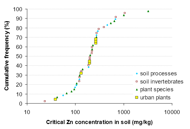
Figure 3. The species sensitivity distribution (plotted as a cumulative frequency against added zinc (Zn) concentration) for soil processes, soil invertebrates and plant species to Zn.
Soil quality guidelines were derived for fresh zinc contamination using three different sets of toxicity data: NOEC and EC10; LOEC and EC30; and EC50. The methods by which they were calculated and the resulting ACL and SQG values are presented in the following sections.
The NOEC and EC10 toxicity data were normalised using the equations presented in Table 5 to the Australian reference soil (Table 6) and then the lowest geometric mean for each species/soil microbial process was entered into the BurrliOZ species sensitivity distribution (Campbell et al. 2000) method. The SSD generated a single numerical value (that is, the ACL(NOEC & EC10) for each desired level of protection. These ACL(NOEC & EC10) values only apply to the Australian reference soil.
The ACL(NOEC & EC10) value for the Australian reference soil with an urban residential land/public open space use was approximately 100 mg/kg. These ACL(NOEC & EC10) values for the reference soil were then used to calculate ACL(NOEC & EC10) values for a range of soils (that is, soil-specific ACL(NOEC & EC10)) for each group of organisms using the same normalisation relationships as before but in the reverse manner. The following explains how the soil-specific ACL(NOEC & EC10) values for soils with an urban residential /public open space land use were calculated as an example of how this was done for each of the land uses.
Soil-specific ACL(NOEC & EC10) values for soil processes varied with soil pH and ranged from 20 to 330 mg/kg added Zn for soils with pHs between 4 and 7.5 (Table 7). The soil-specific ACL(NOEC & EC10) values for invertebrates (Table 8) varied with cation exchange capacity (CEC), with values ranging from 60 to 420 mg/kg for soils with CEC values ranging from 5 to 60 cmolc/kg. Soil-specific ACL(NOEC & EC10) values for plants (Table 9) were pH- and CEC- specific and ranged from 20 to 910 mg/kg for soils with pHs between 4 and 7.5 and CEC values between 5 and 60 cmolc/kg.
Table 7. Soil-specific ACL values for zinc (Zn) based on no observed effect concentration and 10% effect concentration toxicity data that should theoretically protect 80% of soil processes in soils with pH values ranging from 4.0 to 7.5.
Soil pH | Zn ACL (mg/kg) for soil processes |
4.0 | 20 |
4.5 | 30 |
5.0 | 45 |
5.5 | 70 |
6.0 | 100 |
6.5 | 150 |
7.0 | 220 |
7.5 | 330 |
Table 8. Soil-specific ACL values for zinc (Zn) based on no observed effect concentration and 10% effect concentration toxicity data that should theoretically protect 80% of invertebrate species in soils with CEC ranging from 5 to 60 cmolc/kg.
Cation exchange capacity (cmolc/kg) | Zn ACL (mg/kg) for invertebrates |
5 | 60 |
10 | 100 |
20 | 180 |
30 | 240 |
40 | 300 |
60 | 420 |
Table 9. Soil-specific ACL values for zinc (Zn) based on no observed effect concentration and 10% effect concentration toxicity data that should theoretically protect 80% of plant species in soils with pH values ranging from 4.0 to 7.5 and CEC values ranging from 5 to 60 cmolc/kg.
pH | CEC (cmolc/kg) | |||||
| 5 | 10 | 20 | 30 | 40 | 60 |
4.0 | 20 | 30 | 50 | 65 | 75 | 100 |
4.5 | 25 | 40 | 65 | 85 | 110 | 140 |
5.0 | 35 | 55 | 90 | 120 | 140 | 190 |
5.5 | 45 | 75 | 120 | 160 | 200 | 260 |
6.0 | 65 | 100 | 170 | 220 | 270 | 360 |
6.5 | 85 | 140 | 230 | 300 | 370 | 490 |
7.0 | 120 | 190 | 310 | 410 | 500 | 670 |
7.5 | 160 | 260 | 420 | 560 | 690 | 910 |
These soil-specific ACL(NOEC & EC10) values for each organism group (presented in Tables 7 to 9) were then merged into a single set of soil-specific ACL(NOEC & EC10) values—so that the lowest ACL(NOEC & EC10) value for each combination of soil pH and CEC was adopted (Table 10). The ACL(NOEC & EC10) values presented in Table 10 should protect at least 80% of soil processes, soil invertebrate and plant species and these ranged from 20 to 330 mg/kg in soils with pH values between 4 and 7.5 and CEC values between 5 and 60 cmolc/kg. The ACL(NOEC & EC10) values presented in Tables 79 are the ACLs for individual groups of organisms and should not be used as ACL(NOEC & EC10) values.
Table 10. Soil-specific added contaminant limits based on no observed effect concentration and 10% effect concentration toxicity data (ACL(NOEC & EC10), mg/kg) for zinc (Zn) that theoretically protect at least 80% of soil processes, soil invertebrate species and plant species in soils with a pH ranging from 4.0 to 7.5 and CEC values ranging from 5 to 60 cmolc/kg. These values may be used as ACLs(NOEC & EC10) for Zn in freshly contaminated soils with an urban residential /public open space land use.
pH | CEC (cmolc/kg) | |||||
| 5 | 10 | 20 | 30 | 40 | 60 |
4.0 | 20 | 20 | 20 | 20 | 20 | 20 |
4.5 | 25 | 30 | 30 | 30 | 30 | 30 |
5.0 | 35 | 45 | 45 | 45 | 45 | 45 |
5.5 | 45 | 70 | 70 | 70 | 70 | 70 |
6.0 | 60 | 100 | 100 | 100 | 100 | 100 |
6.5 | 60 | 100 | 150 | 150 | 150 | 150 |
7.0 | 60 | 100 | 180 | 220 | 220 | 220 |
7.5 | 60 | 100 | 180 | 240 | 300 | 330 |
The same methods as described above were used to generate the ACL (NOEC & EC10) values for areas of ecological significance and commercial/industrial land uses. The ACL (NOEC & EC10) values for these land uses are presented in Tables 11 and 12.
Table 11. Soil-specific added contaminant limits based on no observed effect concentration and 10% effect concentration toxicity data (ACL(NOEC & EC10), mg/kg) for zinc (Zn) that theoretically protect at least 99% of soil processes, soil invertebrate species and plant species in soils with a pH ranging from 4.0 to 7.5 and CEC values ranging from 5 to 60 cmolc/kg. These values may be used as ACLs(NOEC & EC10) for Zn in freshly contaminated soils for areas of ecological significance.
pH | CEC (cmolc/kg) | |||||
| 5 | 10 | 20 | 30 | 40 | 60 |
4.0 | 4 | 5 | 5 | 5 | 5 | 5 |
4.5 | 6 | 8 | 8 | 8 | 8 | 8 |
5.0 | 8 | 10 | 10 | 10 | 10 | 10 |
5.5 | 10 | 15 | 15 | 15 | 15 | 15 |
6.0 | 15 | 25 | 25 | 25 | 25 | 25 |
6.5 | 15 | 25 | 35 | 35 | 35 | 35 |
7.0 | 15 | 25 | 45 | 55 | 55 | 55 |
7.5 | 15 | 25 | 45 | 60 | 75 | 80 |
Table 12. Soil-specific added contaminant limits based on no observed effect concentration and 10% effect concentration toxicity data (ACL(NOEC & EC10), mg/kg) for zinc (Zn) that theoretically protect at least 60% of soil processes, soil invertebrate species and plant species in soils with a pH ranging from 4.0 to 7.5 and cation exchange capacity (CEC) values ranging from 5 to 60 cmolc/kg. These values may be used as ACLs(NOEC & EC10) for Zn in freshly contaminated soils with a commercial/industrial land use.
pH | CEC (cmolc/kg) | |||||
| 5 | 10 | 20 | 30 | 40 | 60 |
4.0 | 30 | 35 | 35 | 35 | 35 | 35 |
4.5 | 40 | 50 | 50 | 50 | 50 | 50 |
5.0 | 55 | 75 | 75 | 75 | 75 | 75 |
5.5 | 75 | 110 | 110 | 110 | 110 | 110 |
6.0 | 95 | 160 | 160 | 160 | 160 | 160 |
6.5 | 95 | 160 | 240 | 240 | 240 | 240 |
7.0 | 95 | 160 | 280 | 350 | 350 | 350 |
7.5 | 95 | 160 | 280 | 390 | 480 | 520 |
To convert ACLs to SQGs, the ambient background concentration (ABC) needs to be added to the ACL. Three methods of determining the ABC were recommended in the methodology for deriving SQGs (Schedule B5b). The preferred method is to measure the ABC at an appropriate reference site. However, where this is not possible the methods of Olszowy et al. (1995) and Hamon et al. (2004) were recommended, depending on the situation.
For sites with no history of contamination the method of Hamon et al. (2004) was recommended to estimate the ABC. In this method, the ABC for Zn varies with the soil iron concentration (Table 13). Predicted ABC values for Zn range from 3 to 60 mg/kg in soils with iron concentrations between 0.1 and 20%.
Table 13. Zinc (Zn) ABC calculated using the Hamon et al. (2004) method.
Soil iron content (%) | Zn ABC (mg/kg) |
0.1 | 3 |
1 | 10 |
10 | 40 |
20 | 60 |
For aged contaminated sites (i.e. the contamination has been in place for at least two years, see Schedule B5b) the methodology recommends using the 25th percentiles of the ABC data for the ‘old suburbs’ of Olszowy et al. (1995) (see Table 14). The ABC values for Zn in ‘new suburbs’ were similar to the values predicted by the Hamon et al. (2004) method. Therefore it is recommended that the Hamon et al. (2004) method be used to generate ABC values for new suburbs (that is, <2 years old) as soil-specific values will be generated, while for old suburbs with aged contamination (that is, >2 years) it was recommended that the 25th percentile of the ABC data from old suburbs (Olszowy et al. 1995) be used.
Table 14. Zinc (Zn) ABC based on the 25th percentiles of Zn concentrations in ‘old suburbs’ (i.e. >2 years old) from various states of Australia (Olszowy et al. 1995).
Suburb type | 25th percentile of Zn ABC values (mg/kg) | |||
| NSW | QLD | SA | VIC
|
New suburb, low traffic | 25 | 15 | 25 | 15 |
New suburb, high traffic | 45 | 30 | 30 | 20 |
Old suburb, low traffic | 75 | 80 | 55 | 40 |
Old suburb, high traffic | 120 | 160 | 90 | 55 |
To calculate an SQG(NOEC & EC10), the ABC value is added to the ACL(NOEC & EC10). ABC values vary with soil type. Therefore, it is not possible to present a single set of SQG(NOEC & EC10) values. Thus, two examples of SQG(NOEC & EC10) values for urban contaminated soils are provided below. These examples would be at the low and high end of the range of SQGs values (but not the extreme values) generated for Australian soils.
Example 1 |
Site descriptors urban residential/public open space land use in a new suburb. Soil descriptors – a sandy acidic soil (pH 5, CEC 10) with a 1% iron content. The resulting ACL(NOEC & EC10), ABC and SQG(NOEC & EC10) values are: ACL(NOEC & EC10): 45 mg/kg ABC: 10 mg/kg SQG(NOEC & EC10): 55 mg/kg |
Example 2 |
Site descriptors – commercial/industrial land use in a new suburb. Soil descriptors – an alkaline clay soil (pH 7.5, CEC 40) with a 10% iron content. The resulting ACL(NOEC & EC10), ABC and SQG(NOEC & EC10) values are: ACL(NOEC & EC10): 480 mg/kg[1] ABC: 40 mg/kg SQG(NOEC & EC10): 520 mg/kg |
As indicated in the exposure pathway assessment, the log Kd values for Zn measured in a range of Australian soils were below 3 and therefore there is the potential in some soils for Zn to leach to groundwater and effect aquatic ecosystems. Although the calculation of SQGs based on protecting aquatic ecosystems from the effects of leached contaminants is not included in the EIL derivation methodology (Schedule B5b), the calculations are presented here to illustrate the recommended approach and what effect this has on the resulting SQGs. The following SQGs were based on the ACL(NOEC & EC10) values for urban residential/public open space land use.
The soil-specific SQGs for Zn that accounted for leaching potential were calculated using the US EPA method (US EPA 1996).
SQG = Cw . (Kd + (θw + θa . H) / ρb) . DAF (equation 2)
where SQG is the appropriate soil quality guideline in soil (mg/kg), Cw is the target soil leachate concentration (mg/L) (that is, the Australian and New Zealand freshwater quality guideline for Zn, (ANZECC and ARMCANZ 2000)), Kd is the soilwater partition coefficient (L/kg), θw is the water-filled soil porosity Lwater/Lsoil), θa is the air-filled soil porosity (Lair/Lsoil), ρb is the dry soil bulk density (kg/L), H is the Henry’s law constant (unitless), and DAF is the dilution and attenuation factor[2]. The values of DAF used in the calculations were 1 and 20. There is a linear relationship between the DAF and the SQGs, thus the SQGs calculated using a DAF of 20 are 20 times larger than those calculated using a DAF of 1.
The value for θw was set to 0.1 Lwater/Lsoil, θa was set to 0.1 Lair/Lsoil and ρb was set to 1.3 kg/L. The calculated SQG values when DAF was 1 and 20 are presented in Tables 15 and 16 respectively.
Table 15. Soil-specific zinc (Zn) soil quality guidelines (SQG(NOEC & EC10), mg total Zn/kg) based on protecting groundwater ecosystems from groundwater leaching when the dilution and attenuation factor (DAF) was 1.
pH | CEC (cmolc/kg) | |||||
5 | 10 | 20 | 30 | 40 | 60 | |
0.1 | 0.1 | 0.3 | 0.6 | 0.9 | 2 | |
5 | 0.1 | 0.3 | 0.9 | 2 | 2 | 4 |
6 | 0.3 | 0.8 | 2 | 4 | 6 | 10 |
7 | 0.8 | 2 | 6 | 10 | 15 | 30 |
8 | 2 | 5 | 15 | 25 | 40 | 75 |
Table 16. Soil-specific zinc (Zn) soil quality guidelines (SQG(NOEC & EC10), mg total Zn/kg) based on protecting groundwater ecosystems from groundwater leaching when the dilution and attenuation factor (DAF) was 20.
pH | CEC (cmolc/kg) | |||||
5 | 10 | 20 | 30 | 40 | 60 | |
4 | 1 | 2 | 7 | 10 | 20 | 35 |
5 | 2 | 6 | 15 | 30 | 50 | 85 |
6 | 6 | 15 | 45 | 80 | 120 | 220 |
7 | 15 | 40 | 115 | 210 | 310 | 570 |
8 | 40 | 110 | 300 | 530 | 810 | 1500 |
In addition to calculating SQG(NOEC & EC10) values, two other sets of SQGs corresponding to two other levels of protection were generated. T hese were the SQG(LOEC & EC30), which indicate concentrations above which moderate toxic effects would occur and the SQG(EC50), which indicate concentrations above which marked toxic effects would occur.
The Zn SQG(LOEC and EC30) and SQG(EC50) and associated ACL values were calculated using the methodology, except the input data for the SSD was changed to the appropriate type (Table 1). This data is presented in Tables 24 and the raw data can be found in Appendix A. These measures of toxicity were not available in all instances, so, to maximise the data available to calculate SQG(LOEC and EC30) and SQG(EC50) values, the available toxicity data was converted to these measures using conversion factors. The NBRP (cited in Heemsbergen et al. 2008) derived a set of conversion factors for Cu and Zn (Table 17). These experimentally-based conversion factors were used rather than the generic conversion factors presented in Heemsbergen et al. (2008), which is consistent with the approach recommended in the methodology for deriving SQGs. Table 18 shows the ACL(LOEC & EC30) and ACL(EC50) values for the Australian reference soil (that is, a pH of 6 and a CEC of 10 cmolc/kg) with areas of ecological significance, urban residential/public open space and commercial/industrial land uses. The set of soil-specific Zn ACL(LOEC & EC30) and ACL(EC50) values for each land use are presented in Tables 19 and 20.
Table 17. Conversion factors used to convert various measures of toxicity for cations such as copper and zinc. The conversion factors were obtained from unpublished data from the Australian National Biosolids Research Program and were cited by Heemsbergen et al. (2008).
Data being converted | Conversion factor |
NOEC or EC10 to EC50 | x 3 |
NOEC or EC10 to LOEC or EC30 | x 1.5 |
LOEC or EC30 to EC50 | x 2 |
Table 18. Zinc (Zn) added contaminant levels based on lowest observed effect concentration and 30% effect concentration data (ACL(LOEC & EC30)), and based on 50% effect concentration data (ACL(EC50)) for the Australian reference soil with various land uses.
Land use | ACL(LOEC& EC30) values (mg/kg added Zn) | ACL(EC50) values (mg/kg added Zn) |
Areas of ecological significance | 40 | 80 |
Urban residential/public open space | 160 | 290 |
Commercial/industrial | 250 | 450 |
Table 19. Soil-specific added contaminant limits based on lowest observed effect concentration and 30% effect concentration toxicity data (ACL(LOEC & EC30), mg/kg) for fresh zinc (Zn) that should theoretically provide the appropriate level of protection (that is, 99, 80 or 60% of species) to soil processes, soil invertebrate species and plant species in soils with a pH ranging from 4.0 to 7.5 and CEC values ranging from 5 to 60 cmolc/kg. These are the recommended ACL(LOEC & EC30) values in freshly contaminated soils with each land use.
Areas of ecological significance | ||||||
pH | CEC (cmolc/kg) | |||||
5 | 10 | 20 | 30 | 40 | 60 | |
4.0 | 7 | 8 | 8 | 8 | 8 | 8 |
4.5 | 10 | 10 | 10 | 10 | 10 | 10 |
5.0 | 15 | 20 | 20 | 20 | 20 | 20 |
5.5 | 20 | 25 | 25 | 25 | 25 | 25 |
6.0 | 25 | 40 | 40 | 40 | 40 | 40 |
6.5 | 25 | 40 | 60 | 60 | 60 | 60 |
7.0 | 25 | 40 | 70 | 90 | 90 | 90 |
7.5 | 25 | 40 | 70 | 95 | 120 | 130 |
Urban residential/public open space land use | ||||||
pH | CEC (cmolc/kg) | |||||
5 | 10 | 20 | 30 | 40 | 60 | |
4.0 | 25 | 30 | 30 | 30 | 30 | 30 |
4.5 | 35 | 50 | 50 | 50 | 50 | 50 |
5.0 | 50 | 70 | 70 | 70 | 70 | 70 |
5.5 | 70 | 100 | 100 | 100 | 100 | 100 |
6.0 | 90 | 150 | 150 | 150 | 150 | 150 |
6.5 | 90 | 150 | 230 | 230 | 230 | 230 |
7.0 | 90 | 150 | 270 | 340 | 340 | 340 |
7.5 | 90 | 150 | 270 | 370 | 460 | 500 |
Commercial/industrial land use | ||||||
pH | CEC (cmolc/kg) | |||||
5 | 10 | 20 | 30 | 40 | 60 | |
4.0 | 45 | 50 | 50 | 50 | 50 | 50 |
4.5 | 60 | 75 | 75 | 75 | 75 | 75 |
5.0 | 80 | 110 | 110 | 110 | 110 | 110 |
5.5 | 110 | 170 | 170 | 170 | 170 | 170 |
6.0 | 140 | 250 | 250 | 250 | 250 | 250 |
6.5 | 140 | 250 | 360 | 360 | 360 | 360 |
7.0 | 140 | 250 | 420 | 540 | 540 | 540 |
7.5 | 140 | 250 | 420 | 590 | 730 | 800 |
Areas of ecological significance | ||||||
pH | CEC (cmolc/kg) | |||||
5 | 10 | 20 | 30 | 40 | 60 | |
4.0 | 15 | 15 | 15 | 15 | 15 | 15 |
4.5 | 20 | 25 | 25 | 25 | 25 | 25 |
5.0 | 25 | 35 | 35 | 35 | 35 | 35 |
5.5 | 35 | 55 | 55 | 55 | 55 | 55 |
6.0 | 45 | 80 | 80 | 80 | 80 | 80 |
6.5 | 45 | 80 | 110 | 110 | 110 | 110 |
7.0 | 45 | 80 | 130 | 170 | 170 | 170 |
7.5 | 45 | 80 | 130 | 190 | 230 | 250 |
Urban residential/public open space land use | ||||||
pH | CEC (cmolc/kg) | |||||
5 | 10 | 20 | 30 | 40 | 60 | |
4.0 | 50 | 60 | 60 | 60 | 60 | 60 |
4.5 | 70 | 90 | 90 | 90 | 90 | 90 |
5.0 | 95 | 130 | 130 | 130 | 130 | 130 |
5.5 | 130 | 200 | 200 | 200 | 200 | 200 |
6.0 | 170 | 290 | 290 | 290 | 290 | 290 |
6.5 | 170 | 290 | 430 | 430 | 430 | 430 |
7.0 | 170 | 290 | 500 | 640 | 640 | 640 |
7.5 | 170 | 290 | 500 | 690 | 870 | 940 |
Commercial/industrial land use | ||||||
pH | CEC (cmolc/kg) | |||||
5 | 10 | 20 | 30 | 40 | 60 | |
4.0 | 80 | 95 | 95 | 95 | 95 | 95 |
4.5 | 100 | 150 | 150 | 150 | 150 | 150 |
5.0 | 150 | 200 | 200 | 200 | 200 | 200 |
5.5 | 200 | 300 | 300 | 300 | 300 | 300 |
6.0 | 250 | 450 | 450 | 450 | 450 | 450 |
6.5 | 259 | 450 | 650 | 650 | 650 | 650 |
7.0 | 259 | 450 | 750 | 1000 | 1000 | 1000 |
7.5 | 259 | 450 | 750 | 1100 | 1300 | 1400 |
The ABC values for freshly contaminated soils were calculated using the method set out in this Schedule and presented in Table 13.
In order to calculate the SQG(LOEC & EC30) and SQG(EC50) values the soil-specific ABC has to be added to the ACL(LOEC & EC30) and ACL(EC50) values, respectively. Therefore, the SQG(LOEC & EC30) and SQG(EC50) values will always be at least as large as those presented in Tables 19 and 20. Examples of the SQG(LOEC & EC30) and SQG(EC50) values are provided below.
SQG(LOEC & EC30)—Example 1 | |||||||||
Site descriptors urban residential/public open space land use in a new suburb. Soil descriptors – a sandy acidic soil (pH 5, CEC 10) with a 1% iron content. The resulting ACL(LOEC & EC30), ABC and SQG(LOEC & EC30) values are:
|
SQG(LOEC & EC30)—Example 2 | |||||||||
Site descriptors – commercial/industrial land use in a new suburb. Soil descriptors – an alkaline clay soil (pH 7.5, CEC 40) with a 10% iron content. The resulting ACL(LOEC & EC30), ABC and SQG(LOEC & EC30) values are:
|
SQG(EC50)—Example 3 | |||||||||
Site descriptors urban residential/public open space land use in a new suburb. Soil descriptors – a sandy acidic soil (pH 5, CEC 10) with a 1% iron content. The resulting ACL(EC50), ABC and SQG(EC50) values are:
|
SQG(EC50)—Example 4 | |||||||||
Site descriptors commercial/industrial land use in a new suburb. Soil descriptors – an alkaline clay soil (pH 7.5, CEC 40) with a 10% iron content. The resulting ACL(EC50), ABC and SQG(EC50) values are:
|
In addition to calculating SQGs in recently contaminated soils (that is, contamination is <2 years old), an equivalent set of levels was derived for soils where the contamination is aged (that is, it has been present for ≥2 years). The Zn SQG(NOEC & EC10), SQG(LOEC & EC30) and SQG(EC50) for aged sites were calculated using the methods set out in Schedule B5b and this Schedule, the only difference being that laboratory toxicity data based on freshly spiked soils or soils that had not been leached were multiplied by an ageing/leaching factor. A factor (3 for Zn) was developed by Smolders et al. (2009) that accounted for ageing and leaching of various metals. This ageing and leaching factor (ALF) has been incorporated into the methodology to derive the Flemish soil quality guidelines (VLAREBO 2008). Therefore, the raw toxicity data (Appendix A) for Zn that was generated using freshly spiked and non-leached soils was multiplied by this conversion factor and the geometric means for each species and soil process recalculated (Tables 21–23). It should be noted that the values in Tables 21–23 are not simply the data from Tables 2–4 multiplied by 3, as the correction factor was not applied to all the data (for example, data from the field-based NBRP was not adjusted).
The lowest geometric mean of the age-corrected toxicity data for each species/soil microbial process that was used to derive the aged ACL(NOEC & EC10) values is presented in Table 21 for soil processes, Table 22 for soil invertebrate species and Table 23 for plant species. The conversion of the fresh toxicity data to account for ageing/leaching and the resulting toxicity values are presented in Appendix A.
Table 21. The geometric mean values of the aged and age-corrected zinc (Zn) toxicity data (expressed in terms of added Zn) for soil processes.
Soil process | Geometric means (mg/kg added Zn) | ||
| EC10 or NOEC | EC30 or LOEC | EC50 |
Acetate decomposition | 561 | 841 | 1681 |
Amidase | 363 | 545 | 1091 |
Ammonification | 295 | 443 | 885 |
Arylsulphatase | 868 | 1303 | 2605 |
Glucose decomposition | 274 | 1169 | 2904 |
Nitrate reductase | 168 | 252 | 504 |
Nitrification | 455 | 706 | 930 |
Phosphatase | 2022 | 3033 | 6066 |
Respiration | 313 | 470 | 940 |
Table 22. The geometric mean values of the aged and age-corrected zinc (Zn) toxicity data (expressed in terms of added Zn) for soil invertebrate species.
Invertebrate species | Geometric means (mg/kg added Zn) | |||
Common name | Scientific name | EC10 or NOEC | EC30 or LOEC | EC50 |
Earthworm | A. caliginosa | 669 | 823 | 1172 |
Earthworm | A. rosea | 1172 | 1221 | 1308 |
Earthworm | E. fetida | 602 | 888 | 1726 |
Earthworm | L. rubellus | 659 | 855 | 1328 |
Earthworm | L. terrestris | 3187 | 3771 | 5026 |
Nematode | Acrobeloides sp. | 663 | 995 | 1989 |
Nematode | C. elegans | 366 | 550 | 1099 |
Nematode | C. elegans (dauer larval stage) | 2068 | 3103 | 6205 |
Nematode | Community nematodes | 919 | 1378 | 2756 |
Nematode | Eucephalobus sp. | 404 | 605 | 1210 |
Nematode | Plectus sp. | 70 | 105 | 210 |
Nematode | Rhabditidae sp. | 597 | 896 | 1791 |
Potworm | E. albidus | 363 | 544 | 1088 |
Potworm | E. crypticus | 828 | 1241 | 2483 |
Springtail | F. candida | 566 | 848 | 1696 |
Table 23. The geometric mean values of the aged and age-corrected zinc (Zn) toxicity data (expressed in terms of added Zn) for plant species.
Species | Scientific name | Geometric means (mg/kg added Zn) | ||
|
| EC10 or NOEC | EC30 or LOEC | EC50 |
Alfalfa | M. sativa | 595 | 892 | 1784 |
Barley | H. vulgare | 110 | 306 | 652 |
Beet | B.vulgaris | 595 | 892 | 1784 |
Black or white lentil | V. mungo | 284 | 426 | 852 |
Canola | B. napus | 230 | 328 | 409 |
Common vetch | V. sativa | 127 | 190 | 380 |
Cotton | Gossypium sp. | 272 | 288 | 293 |
Fenugreek | T. foenum graecum | 318 | 477 | 953 |
Lettuce | L. sativa | 793 | 1189 | 2379 |
Maize | Z. mays | 460 | 694 | 1324 |
Millet | P. milaceum | 540 | 1580 | 2026 |
Oats | A. sativa | 667 | 1000 | 2000 |
Onion | A. cepa | 198 | 297 | 594 |
Pea | P. sativum | 793 | 1189 | 2379 |
Peanuts | A. hypogaea | 140 | 224 | 280 |
Red clover | T. pratense | 117 | 176 | 351 |
Sorghum | Sorghum sp. | 256 | 528 | 924 |
Spinach | S. oleracea | 396 | 595 | 1189 |
Sugar cane | Sacharum | 3220 | 4830 | 9661 |
Tomato | L. esculentum | 793 | 1189 | 2379 |
Triticale | Tritosecale sp. | 998 | 1364 | 1658 |
Wheat | T. aestivum | 640 | 928 | 1172 |
For each urban residential/public open space land use, soil-specific ACL(NOEC & EC10) values were derived separately for soil processes, soil invertebrate species and plant species (data not shown). Within each land use type, the soil-specific ACL(NOEC & EC10) values for each organism group were then merged so that the lowest ACL(NOEC & EC10) value for each combination of soil pH and CEC was adopted (Table 24). These should theoretically protect 99%, 80% and 60% of all soil processes, soil invertebrate species and plant species that are exposed to aged Zn contamination in soils that are in an area of ecological significance, or have an urban residential/public open space, commercial/industrial land use, respectively.
Table 24. Soil-specific added contaminant limits based on no observed effect concentration and 10% effect concentration toxicity data (ACL(NOEC & EC10), mg/kg) for aged zinc (Zn) contamination that should theoretically provide the appropriate level of protection (i.e. 99, 80 or 60% of species) to soil processes, soil invertebrate species and plant species in soils with a pH ranging from 4.0 to 7.5 and CEC values ranging from 5 to 60 cmolc/kg. These are the recommended ACL(NOEC & EC10) values for Zn in aged contaminated soils with each land use.
Areas of ecological significance | ||||||
pH | CEC (cmolc/kg) | |||||
5 | 10 | 20 | 30 | 40 | 60 | |
4.0 | 10 | 10 | 10 | 10 | 10 | 10 |
4.5 | 15 | 20 | 20 | 20 | 20 | 20 |
5.0 | 20 | 25 | 25 | 25 | 25 | 25 |
5.5 | 25 | 40 | 40 | 40 | 40 | 40 |
6.0 | 35 | 55 | 55 | 55 | 55 | 55 |
6.5 | 35 | 55 | 85 | 85 | 85 | 85 |
7.0 | 35 | 55 | 100 | 125 | 125 | 125 |
7.5 | 35 | 55 | 100 | 130 | 170 | 180 |
Urban residential/public open space land use | ||||||
pH | CEC (cmolc/kg) | |||||
5 | 10 | 20 | 30 | 40 | 60 | |
4.0 | 45 | 55 | 55 | 55 | 55 | 55 |
4.5 | 60 | 80 | 80 | 80 | 80 | 80 |
5.0 | 85 | 110 | 110 | 110 | 110 | 110 |
5.5 | 110 | 170 | 170 | 170 | 170 | 170 |
6.0 | 150 | 250 | 250 | 250 | 250 | 250 |
6.5 | 150 | 250 | 370 | 370 | 370 | 370 |
7.0 | 150 | 250 | 440 | 550 | 550 | 550 |
7.5 | 150 | 250 | 440 | 600 | 750 | 800 |
Commercial/industrial land use | ||||||
pH | CEC (cmolc/kg) | |||||
5 | 10 | 20 | 30 | 40 | 60 | |
4.0 | 70 | 85 | 85 | 85 | 85 | 85 |
4.5 | 100 | 120 | 120 | 120 | 120 | 120 |
5.0 | 125 | 180 | 180 | 180 | 180 | 180 |
5.5 | 180 | 270 | 270 | 270 | 270 | 270 |
6.0 | 230 | 400 | 400 | 400 | 400 | 400 |
6.5 | 230 | 400 | 590 | 590 | 590 | 590 |
7.0 | 230 | 400 | 690 | 870 | 870 | 870 |
7.5 | 230 | 400 | 690 | 940 | 1200 | 1300 |
The ABC values for aged Zn contamination used to calculate aged SQG(LOEC and EC30) and SQG(EC50) values were obtained from Olszowy et al. (1995) and are presented in Table 14.
SQGs are the sum of the ABC and ACL values, both of which are soil-specific. It is, therefore, not possible to present a single set of aged SQGs. Thus, some examples of aged SQGs for aged urban contaminated soils are provided below. The presented examples represent SQGs that would be at the low and high end of the range of SQGs that would be generated for Australian soils, but are not extreme values.
Example 1 | |||||||||
Site descriptors – urban residential/public open space land use in an old NSW suburb with low traffic volume. Soil descriptors – a sandy acidic soil (pH 5, CEC 10) with 1% iron and aged Zn contamination. The resulting ACL(NOEC & EC10), ABC and SQG(NOEC & EC10) values are:
|
Example 2 | |||||||||
Site descriptors – commercial/industrial land use in an old Queensland suburb with a high traffic volume. Soil descriptors – an alkaline clay soil (pH 7.5, CEC 40) with a 10% iron and aged Zn contamination. The resulting ACL(NOEC & EC10), ABC and SQG(NOEC & EC10) values are:
|
The Zn SQG(LOEC & EC30) and SQG(EC50) values for aged sites were calculated using the method described in this Schedule with the exception that aged or age-corrected Zn toxicity data was used (Tables 21–23). Table 25 presents the ACL(LOEC & EC30) and ACL(EC50) values for the Australian reference soil (Table 6) for areas of ecological significance, urban residential/public open space, and commercial/industrial land uses.
The soil-specific ACL(LOEC and EC30) and ACL(EC50) values for aged Zn contamination and the various land uses are presented in Tables 26 and 27 respectively. As with the ACL(NOEC & EC10) values for aged Zn contamination, the ACL(LOEC & EC30) and ACL(EC50) values must have the soil-specific ABC added. Therefore, the SQG(LOEC & EC30) and SQG(EC50) values will be larger than the corresponding ACL values presented in Tables 26 and 27, respectively. Examples of the SQG(LOEC & EC30) and SQG(EC50) values are provided below.
Table 25. Zinc (Zn) ACLs for the Australian reference soil (pH = 6, CEC = 10 cmolc/kg) based on lowest observed effect concentration and 30% effect concentration toxicity data, and based on 50% effect concentration toxicity data.
Land use | ACL(LOEC & EC30) values (mg/kg added Zn) | ACL(EC50) values (mg/kg added Zn) |
Areas of ecological significance | 90 | 140 |
Urban residential/public open space | 400 | 700 |
Commercial/industrial | 630 | 1100 |
Table 26. Soil-specific added contaminant limits based on lowest observed effect concentration and 30% effect concentration toxicity data (ACL(LOEC & EC30), mg/kg) for aged zinc (Zn) contamination that should theoretically provide the appropriate level of protection (i.e. 99, 80 or 60% of species) to soil processes, soil invertebrate species and plant species in soils with a pH ranging from 4.0 to 7.5 and CEC values ranging from 5 to 60 cmolc/kg. These are the recommended ACL(LOEC & EC30) values for Zn in aged contaminated soils with each land use.
Areas of ecological significance | ||||||
pH | CEC (cmolc/kg) | |||||
5 | 10 | 20 | 30 | 40 | 60 | |
4.0 | 15 | 20 | 20 | 20 | 20 | 20 |
4.5 | 20 | 25 | 25 | 25 | 25 | 25 |
5.0 | 30 | 40 | 40 | 40 | 40 | 40 |
5.5 | 40 | 60 | 60 | 60 | 60 | 60 |
6.0 | 50 | 90 | 90 | 90 | 90 | 90 |
6.5 | 50 | 90 | 130 | 130 | 130 | 130 |
7.0 | 50 | 90 | 150 | 190 | 190 | 190 |
7.5 | 50 | 90 | 150 | 210 | 260 | 280 |
Urban residential/public open space land use | ||||||
pH | CEC (cmolc/kg) | |||||
5 | 10 | 20 | 30 | 40 | 60 | |
4.0 | 70 | 85 | 85 | 85 | 85 | 85 |
4.5 | 100 | 120 | 120 | 120 | 120 | 120 |
5.0 | 130 | 180 | 180 | 180 | 180 | 180 |
5.5 | 180 | 270 | 270 | 270 | 270 | 270 |
6.0 | 230 | 400 | 400 | 400 | 400 | 400 |
6.5 | 230 | 400 | 590 | 590 | 590 | 590 |
7.0 | 230 | 400 | 700 | 880 | 880 | 880 |
7.5 | 230 | 400 | 700 | 960 | 1200 | 1300 |
Commercial/industrial land use | ||||||
pH | CEC (cmolc/kg) | |||||
5 | 10 | 20 | 30 | 40 | 60 | |
110 | 130 | 130 | 130 | 130 | 130 | |
4.5 | 150 | 190 | 190 | 190 | 190 | 190 |
5.0 | 210 | 290 | 290 | 290 | 290 | 290 |
5.5 | 280 | 420 | 420 | 420 | 420 | 420 |
6.0 | 360 | 620 | 620 | 620 | 620 | 620 |
6.5 | 360 | 620 | 920 | 920 | 920 | 920 |
7.0 | 360 | 620 | 1100 | 1400 | 1400 | 1400 |
7.5 | 360 | 620 | 1100 | 1500 | 1900 | 2000 |
Table 27. Soil-specific added contaminant limits based on 50% effect concentration toxicity data (ACL(EC50), mg/kg) for aged zinc (Zn) contamination that should theoretically provide the appropriate level of protection (i.e. 99, 80 or 60% of species) to soil processes, soil invertebrate species and plant species in soils with a pH ranging from 4.0 to 7.5 and cation exchange capacity (CEC) values ranging from 5 to 60 cmolc/kg. These are the recommended ACL(EC50) values for Zn in aged contaminated soils with each land use.
Areas of ecological significance | ||||||
pH | CEC (cmolc/kg) | |||||
5 | 10 | 20 | 30 | 40 | 60 | |
4.0 | 25 | 30 | 30 | 30 | 30 | 30 |
4.5 | 35 | 45 | 45 | 45 | 45 | 45 |
5.0 | 45 | 65 | 65 | 65 | 65 | 65 |
5.5 | 65 | 95 | 95 | 95 | 95 | 95 |
6.0 | 85 | 140 | 140 | 140 | 140 | 140 |
6.5 | 85 | 140 | 210 | 210 | 210 | 210 |
7.0 | 85 | 140 | 250 | 310 | 310 | 310 |
7.5 | 85 | 140 | 250 | 340 | 430 | 460 |
Urban residential/public open space land use | ||||||
pH | CEC (cmolc/kg) | |||||
5 | 10 | 20 | 30 | 40 | 60 | |
4.0 | 130 | 150 | 150 | 150 | 150 | 150 |
4.5 | 170 | 220 | 220 | 220 | 220 | 220 |
5.0 | 230 | 330 | 330 | 330 | 330 | 330 |
5.5 | 320 | 480 | 480 | 480 | 480 | 480 |
6.0 | 410 | 710 | 710 | 710 | 710 | 710 |
6.5 | 410 | 710 | 1100 | 1100 | 1100 | 1100 |
7.0 | 410 | 710 | 1200 | 1600 | 1600 | 1600 |
7.5 | 410 | 710 | 1200 | 1700 | 2100 | 2300 |
Commercial/industrial land use | ||||||
pH | CEC (cmolc/kg) | |||||
5 | 10 | 20 | 30 | 40 | 60 | |
4.0 | 200 | 230 | 230 | 230 | 230 | 230 |
4.5 | 270 | 350 | 350 | 350 | 350 | 350 |
5.0 | 370 | 510 | 510 | 510 | 510 | 510 |
5.5 | 510 | 760 | 760 | 760 | 760 | 760 |
6.0 | 650 | 1100 | 1100 | 1100 | 1100 | 1100 |
6.5 | 650 | 1100 | 1700 | 1700 | 1700 | 1700 |
7.0 | 650 | 1100 | 1900 | 2500 | 2500 | 2500 |
7.5 | 650 | 1100 | 1900 | 2700 | 3400 | 3600 |
The ABC values used for aged Zn contamination are presented in Table 14.
Both the ACL and ABC values for aged zinc contamination are soil-specific therefore a single set of SQGs could not be presented. Thus, examples from the low and high portions of the range of SQG(LOEC & EC30) and SQG(EC50) are presented below.
SQG(LOEC & EC30)—Example 1 | |||||||||
Site descriptors urban residential/public open space land use in an old NSW suburb with low traffic volume. Soil descriptors – a sandy acidic soil (pH 5, CEC 10) with 1% iron content. The resulting ACL(LOEC & EC30), ABC and SQG(LOEC & EC30) values are:
This SQG(LOEC & EC30) would then be rounded off using the rules in section 2.1 to a value of 250 mg/kg. |
SQG(LOEC & EC30)—Example 2 | |||||||||
Site descriptors commercial/industrial land use in an old Victorian suburb with high traffic volume. Soil descriptors – an alkaline clay soil (pH 7.5, CEC 40) with a 10% iron content. The resulting ACL(LOEC & EC30), ABC and SQG(LOEC & EC30) values are:
This SQG(LOEC & EC30) would then be rounded off using the rules in section 2.1 to a value of 2000 mg/kg. |
SQG(EC50)—Example 3 | |||||||||
Site descriptors urban residential/public open space land use in an old NSW suburb with low traffic volume. Soil descriptors – a sandy acidic soil (pH 5, CEC 10) with 1% iron content. The resulting ACL(EC50), ABC and SQG(EC50) values are:
This SQG(EC50) would then be rounded off using the rules in section 2.1 to a value of 400 mg/kg.
|
SQG(EC50)—Example 4 | |||||||||
Site descriptors commercial/industrial land use in an old Victorian suburb with high traffic volume. Soil descriptors – an alkaline clay soil (pH 7.5, CEC 40) with a 10% iron content. The resulting ACL(EC50), ABC and SQG(EC50) values are:
This SQG(EC50) would then be rounded off using the rules in section 2.1 to a value of 3500 mg/kg. |
Based on the criteria established in the methodology for SQG derivation (Schedule B5b), the Zn SQGs were considered to be of high reliability. This occurred as the toxicity data set easily met the minimum data requirements to use the SSD method and normalisation relationships were available to account for soil characteristics.
A compilation of SQGs for Zn from a number of jurisdictions is presented in Table 28. These SQGs have a variety of purposes and levels of protection and therefore comparison of the SQGs between each other and with the Zn SQGs is problematic. The guidelines for Zn range from 20 mg/kg (added Zn) for the Netherlands to 200 mg/kg (total Zn) for Canada. The superseded interim urban EIL (NEPC 1999) was 200 mg/kg total Zn and therefore at the top of the range of the international Zn guidelines.
The Zn ACL(NOEC & EC10) values in freshly contaminated urban residential/public open space soils ranged from 20330 mg/kg (added Zn) (Table 10). The corresponding values for urban residential/public open space soils with aged Zn contamination ranged from 45810 mg/kg (Table 24). The lowest ACLs (for sandy acidic soils) were very similar to the lowest of the international SQGs, but considerably lower than the superseded interim urban EIL. However, the largest ACLs (for neutral to alkaline, high CEC soils) were considerably larger than any of the international SQGs apart from the Dutch intervention level, which has a different purpose from the ACLs. Thus, in soils where the Zn has a low bioavailability, higher concentrations of Zn are permitted under the methodology than under the superseded interim urban EIL.
The intervention value in the Netherlands is 720 mg/kg total Zn. The range of ACL(EC50) values (which most closely relate to the Dutch intervention value) in freshly contaminated urban residential/public open space soils was 50940 mg/kg (Table 20). While the range for aged Zn contamination was 1252,300 mg/kg (Table 27), the Dutch value corresponds to the 60th and 25th percentile of the range of ACL(EC50) values for fresh and aged Zn contamination respectively. Therefore, depending on soil physicochemical properties, the ACL(EC50) values would permit considerably less (in high bioavailability soils) to considerably more (in low bioavailability soils) Zn than in the Netherlands.
Table 28. Soil quality guidelines for zinc (Zn) from international jurisdictions.
Name of zinc limit | Numerical value of the limit (mg/kg) |
Dutch intervention level1 | 720 (added Zn) |
Dutch maximum permissible addition1 | 20 (added Zn) |
Canadian SQG (residential)2 | 200 (total Zn) |
Eco-SSL plants3 | 160 (total Zn) |
Eco-SSL soil invertebrates3 | 120 (total Zn) |
Eco-SSL avian3 | 46 (total Zn) |
Eco-SSL mammalian3 | 79 (total Zn) |
EU soil guidelines using negligible risk4 | 67150 (total Zn) |
1 = VROM, 2000
2 = CCME, 1999a and 2006 and http://www.ccme.ca/publications/list_publications.html#link2
3 = http://www.epa.gov/ecotox/ecossl/
4 = Carlon, 2007
The metalloid As occurs in a number of oxidation states: -3 (-III), 0, +3 (III) and +5 (V). Arsenic (III) is the dominant form under reducing conditions and As (V) is the dominant form in oxidised soils. The SQG derivation methodology (Schedule B5b) is only suitable for the aerobic portion of soils. SQGs for As were therefore calculated using only well oxidised soil studies. Therefore, arsenic will predominantly be present as As (V) but, as all the toxicity studies expressed toxicity in terms of total arsenic, the SQGs generated in this study are for total arsenic. For waterlogged soils, a separate As SQG should be derived, due to the difference between As (III) and As (V) in both toxicity and bioavailability in these soils. The chemical abstract service number (a unique identification number for each chemical) for As is 7440-38-2.
The two key considerations in determining the most important exposure pathways for inorganic contaminants such as As are whether they biomagnify and whether they have the potential to leach to groundwater. A surrogate measure of the potential for a contaminant to leach is its watersoil partition coefficient (Kd). If the logarithm of the Kd (log Kd) of an inorganic contaminant is less than 3 then it is considered to have the potential to leach to groundwater (Schedule B5b). The log Kd reported by Crommentuijn et al. (2000) was 2.28 L/kg, so As has the potential in some soils to leach to groundwater. This is consistent with information regarding human health problems experienced in Bangladesh from the presence of As in groundwater. The methodology for EIL derivation (Schedule B5b) does not advocate the routine derivation of EILs that account for leaching potential. Rather, it advocates that this is done on a site-specific basis as appropriate. However, the calculations are presented here to illustrate the recommended approach and the effect that this would have on the resulting SQGs.
Arsenic is not known to biomagnify in oxidised soils (Heemsbergen et al. 2009) and therefore only direct toxicity routes of exposure were considered in deriving the SQGs.
The raw toxicity data for As is presented in Appendix B. The toxicity data (geometric means for each species) used to calculate the SQGs is presented in Table 29. There was toxicity data for three soil invertebrate species, five terrestrial animal species and 13 species of plants. These meet the minimum data requirements recommended by Heemsbergen et al. (2008) to use the BurrliOZ SSD method (Campbell et al. 2000).
Table 29. Geometric mean values of arsenic (As) toxicity data (expressed in terms of total As) for soil invertebrate species, terrestrial bird and mammal species and plant species.
Test species | Geometric mean (mg/kg) | |||
Common name | Scientific name | EC10 or NOEC | EC30 or LOEC | EC50 |
Bean | Phaseolus vulgaris | 22.6 | 84 | 168 |
Blueberry | Vaccinium sp. | 22.2 | 55 | 111 |
Common rat | Rattus norvegicus | 10.0 | 25 | 50 |
Corn | Z. mays | 25.1 | 67 | 123 |
Cotton | Gossypium sp. | 20.8 | 52 | 104 |
Deer mouse | Peromyscus maniculatus | 320 | 1600 | 1600 |
Earthworm | Eisenia fetida | 20.0 | 100 | 100 |
Earthworm | L. rubellus | 76.1 | 381 | 381 |
Earthworm | L. terrestris | 100 | 250 | 500 |
Fulvous whistling duck | Dendrocygna bicolour | 229 | 1145 | 1145 |
Grass |
| 13.4 | 81 | 161 |
Northern bobwhite | Colinus virginianus | 54.0 | 270 | 270 |
Oat | A. sativa | 22.7 | 44 | 70 |
Pea | Pisum sativum | 20.8 | 52 | 104 |
Pine |
| 292 | 731 | 1462 |
Potato | Solanum tuberosum | 36.3 | 108 | 181 |
Radish | Raphanus sativa | 67.7 | 169 | 339 |
Sheep | Ovis aries | 25.0 | 63 | 125 |
Soyabean | Glycine max | 9.7 | 24 | 35 |
Tomato | L. esculentum | 62.5 | 166 | 263 |
Wheat | T. aestivum | 43.4 | 153 | 307 |
In order to maximise the use of the available toxicity data, conversion factors (adopted from the Australian and New Zealand guidelines for fresh and marine water quality (ANZECC & ARMCANZ 2000) by Heemsbergen et al. (2008)) were used to permit the inter-conversion of NOEC, LOEC, EC50, EC30 and EC10 data. Conversion factors for cations (for example, Cu and Zn) were developed by the NBRP and recommended by Heemsbergen et al. (2008) in preference to the default conversion factors adopted from the WQGs. However, as As is predominantly found in anionic form in soils, the default conversion factors were used (Table 30).
Table 30. The default conversion factors used to convert different measures of toxicity to chronic no observed effect concentrations (NOECs) or 10% effect concentrations (EC10). Sourced from Heemsbergen et al. (2008), who adopted the values from the Australian and New Zealand guidelines for fresh and marine water quality (ANZECC & ARMCANZ 2000).
Toxicity dataa | Conversion factor |
EC50 to NOEC or EC10 | 5 |
LOEC or EC30 to NOEC or EC10 | 2.5 |
MATC* to NOEC or EC10 | 2 |
a EC50 is the concentration that causes a 50% effect, EC30 is the concentration that causes a 30% effect, EC10 is the concentration that causes a 10% effect, NOEC = no observed effect concentration, LOEC = lowest observed effect concentration, *MATC = the maximum acceptable toxicant concentration and is the geometric mean of the NOEC and LOEC.
It is well known that soil physicochemical properties affect the toxicity and bioavailabiity of As. However, this knowledge is qualitative. For example, Sheppard (1992) reviewed the existing literature and concluded that the toxicity of As was five times more toxic in sands and loams than in clay soils. There is only one set of published normalisation relationships for As toxicity (Song et al. 2006). This relates the toxicity of As (i.e. barley root elongation) expressed in terms of total added As, ammonium sulphate [(NH4)2SO4]-extractable As or ammonium phosphate (NH4H2PO4)-extractable As to soil properties such as oxalate-extractable Mn and oxalate-extractable Fe concentrations. The normalisation relationships for EC10 and EC50 toxicity data expressed in terms of total added As (from Song et al. 2006) are:
EC10 = 0.1 (oxalate-extractable Mn) + 1.03 (% clay) – 9.25 (equation 3)
(r2 adj = 0.89, p = <0.001, n = 16)
EC50 = 0.21 (oxalate-extractable Mn) + 0.016 (oxalate-extractable Fe)
+ 4.29 (% clay) – 48.2 (equation 4)
(r2 adj = 0.91, p = <0.001, n = 16)
However, with the exception of the Song et al. (2006) data, none of the available As toxicity studies had expressed the toxicity in the units of the normalisation relationships nor had the studies measured the soil properties used in the normalisation relationships. Therefore, the normalisation relationships could not be used.
Figure 4 shows the SSD (that is, the cumulative distribution of the geometric means of species sensitivities to As) for all species for which As toxicity data was available. The distribution of the major groups of organisms along the SSD is uniform—thus all of the organism groups have a smilar sensitivity to As.
Figure 4. The species sensitivity distribution (plotted as a cumulative frequency against total arsenic (As) concentration) of As for soil invertebrate species, terrestrial vertebrate species and plant species.

The As toxicity data could not be normalised to the Australian reference soil because none of the publications had reported the properties required by the one normalisation relationship available for As. Thus, soil-specific ACLs could not be derived. Rather, a single generic ACL for each land use was derived. These generic ACLs would apply to all Australian soils of the appropriate land use. For example, the single ACL for urban residential /public open space land use would apply to all Australian urban residential/public open space soils.
All the available As toxicity data (apart from that of Song et al. 2006) were reported as total concentrations without making a distinction between added and background concentrations. The Hamon et al. (2004) method can predict the ABC for As in Australian soils. For European soils or toxicity studies, the Dutch background standardisation equation for As can be used (Lexmond et al. 1986):
As= 0.4*(clay content + organic matter content) (equation 5)
However, the As toxicity studies did not report the Fe and Mn contents (required by the Hamon et al., 2004 method) or the organic matter or clay content (required by the Lexmond et al. 1986 method) of the soils in which the toxicity was determined. Therefore, it was not possible to estimate the ABC nor express toxicity in terms of added concentrations. As a result, no ACL values could be calculated.
The situation for As was that:
Therefore, only a single numerical value was generated by the BurrliOZ SSD method for each of the three land uses (that is, areas of ecological significance, urban residential/public open space, and commercial/industrial).
The output was the SQG(NOEC & EC10) for that particular land use and no soil-specific SQG(NOEC & EC10) values could be calculated. The As SQG(NOEC & EC10) values for the three land uses are presented in Table 31.
Table 31. Generic soil quality guidelines based on no observed effect concentration and 10% effect concentration toxicity data (SQG(NOEC & EC10)) for fresh arsenic (As) contamination in soil with different land uses.
Land use | SQG(NOEC & EC10) (mg/kg total As) |
Areas of ecological significance | 8 |
Urban residential/public open space | 20 |
Commercial/industrial | 30 |
It should be noted, because As has generic SQG(NOEC & EC10) values, that they should be applied to all Australian soils that have the particular land use.
Despite the fact that ACLs could not be derived for As, the issue of background concentrations of As in Australian soils will be discussed as the situation could change in the future if additional data becomes available. If, in the future, toxicity data can be expressed in terms of added concentrations, it is recommended that the method of Hamon et al. (2004) be used to derive ABC values. Examples of the ABC values generated by the Hamon et al. (2004) method are presented in Table 32. The soil-specific estimate of ABC could be added to a generic ACL (if toxicity data could be expressed as added As, but no normalisation relationships were suitable) or it could be added to a soil-specific ACL (if it were possible to express the toxicity data in terms of added As and if normalisation relationships could be applied to the data).
Table 32. Ambient background concentrations of arsenic (As) estimated using the method of Hamon et al. (2004) as a function of the iron content of the soil.
Soil iron (%) | As (mg/kg) |
0.1 | 1 |
1 | 3 |
10 | 12 |
20 | 18 |
The log Kd value for As (Crommentuijn et al. 2000) was below 3 and therefore in accordance with the SQG derivation methodology (Schedule B5b) SQG(NOEC & EC10) values were derived to protect aquatic ecosystems from the effects of leached As from freshly contaminated soils.
The As SQG(NOEC & EC10) values based on protecting groundwater ecosystems were calculated using the US EPA method (US EPA 1996). The generic SQG(NOEC & EC10) values were calculated using DAF values of one and 20 and these are presented in Table 33. There is a linear relationship between the DAF and the SQGs, thus the SQGs calculated using a DAF of 20 are 20 times larger than those calculated using a DAF of 1.
Table 33. Generic arsenic (As) soil quality guidelines (SQGs, mg total As/kg) based on no observed effect concentration and 10% effect concentration toxicity data to protect groundwater ecosystems from leaching.
Dilution factor | 1 | 20 |
SQG (mg/kg) | 4.6 | 91 |
The SQG(LOEC & EC30) and SQG(EC50) values were calculated using the same method as for the As SQG(NOEC & EC10) values ,except that different toxicity data was used. The data used is presented in Table 29. To maximise the data available to generate the SQG(LOEC & EC30) and SQG(EC50) values, the available toxicity data was converted to the appropriate measure of toxicity using the default conversion factors presented in Table 30.
As with the SQG(NOEC & EC10) values for As, soil-specific SQG(LOEC & EC30) and SQG(EC50) values could not be generated, but rather a single generic SQG(LOEC & EC30) and SQG(EC50) value was generated for each of the three land uses (Table 34). Also, all toxicity data was expressed as total As rather than added As. As these are generic SQG(LOEC & EC30) and SQG(EC50) values ,they should be applied to all Australian soils with a particular land use.
Table 34: Generic soil quality guidelines based on lowest observed effect concentration and 30% effect concentration toxicity data (SQG(LOEC & EC30)), and based on 50% effect concentration toxicity data (SQG(EC50)) for soil with different land uses.
Land use | SQG(LOEC & EC30) (mg/kg total As) | SQG(EC50) (mg/kg total As) |
Areas of ecological significance | 20 | 30 |
Urban residential/public open space | 50 | 90 |
Commercial/industrial | 80 | 140 |
Song et al. (2006) conducted some experiments to determine the effect of ageing As over three months in four soils. They found that in all soils the toxicity and extractability decreased and the extent of the decrease ranged from 2- to 12-fold (Song et al. 2006). Yang et al. (2002) and Fendorf et al. (2004) also found that As aged in soils with the majority occurring within the first few months. Yang et al. (2002) also found that As ageing did not always occur—it occurred in only 47% (i.e. 17 out of 36) of the soils they examined. Song et al. (2006) found that the extent of ageing was significantly correlated with oxalate-extractable iron and Olsen-P concentrations in the four test soils. However, they also noted that data on more soils was needed in order for the relationships to be considered more robust. Song et al. (2006) concluded that ageing of As ‘should be taken into account during risk assessment’. Therefore, in order to account for ageing in a conservative manner (that is, one that is protective of the environment), the lowest ALF factor (2) determined by Song et al. (2006) was used to derive the aged SQGs. This ALF was applied to all the toxicity data.
As the available toxicity data can only be expressed as total As concentrations, ACL values could not be derived, so SQGs were derived. The ALF of 2 was applied to all the toxicity data; therefore the aged SQG(NOEC & EC10), SQG(LOEC & EC30) and SQG(EC50) values are exactly twice the corresponding fresh SQGs for arsenic. The resulting aged SQG(NOEC & EC10), SQG(LOEC & EC30) and SQG(EC50) values are presented in Table 35.
Land use | SQG(NOEC & EC10) (mg/kg total As) | SQG(LOEC & EC30) (mg/kg total As) | SQG(EC50) (mg/kg total As) |
Areas of ecological significance | 15 | 40 | 60 |
Urban residential/public open space | 40 | 100 | 180 |
Commercial/industrial | 60 | 160 | 290 |
Background levels of As are not elevated by historic pollution in urban residential/public open space soils, as can be seen by data from Olszowy et al. (1995) (Table 36). Therefore, in the future, if toxicity data can be expressed in terms of added concentrations, it is recommended that the method of Hamon et al. (2004) be used to estimate background values, as they are soil-specific. Examples of the ABC values generated by the Hamon et al. (2004) method are presented in Table 32.
Table 36. Background concentrations of arsenic (As) from Olszowy et al. (1995) in suburbs of different age and with different intensities of traffic in various states of Australia.
Suburb type | 25th percentile As (mg/kg) | |||
| NSW | QLD | SA | VIC |
New suburb, low traffic | 5 | 3 | 5 | NA |
New suburb, high traffic | 5 | 3 | 5 | NA |
Old suburb, low traffic | 5 | 4 | 5 | 5 |
Old suburb, high traffic | 5 | 3 | 5 | 5 |
NA = not available
The As toxicity dataset met the minimum data requirements to use the SSD method but there were no normalisation relationships available to account for soil characteristics. Based on the criteria for assessing the reliability of SQGs (Schedule B5b), this means that the As SQGs were considered to be of moderate reliability.
A compilation of SQGs for As from a number of jurisdictions is presented in Table 37. These guidelines have a variety of purposes and levels of protection and therefore comparison of the values is problematic. The SQGs for As range from 4.5 mg/kg (added As) for the Dutch to 110 mg/kg (total As) for another European country. The superseded interim urban EIL (NEPC 1999) was 20 mg/kg total As and lies in the lower portion of the range of As SQGs. The As SQG(NOEC & EC10) for freshly contaminated urban residential/public open space soils was 20 mg/kg (total As) and thus identical to the superseded interim urban EIL. The SQG(NOEC & EC10) for aged contamination at 40 mg/kg is twice the superseded interim urban EIL for As.
The SQG(LOEC & EC30) and SQG(EC50) values for As in freshly contaminated urban residential/public open space soils are 50 and 80 mg/kg respectively. The SQG(LOEC & EC30) is in the middle of the range of SQGs for other jurisdictions, while the SQG(EC50) is in the upper portion of the range of SQGs. The aged As SQG(LOEC & EC30) for urban residential/public open space soils lies in the upper part of the range of international SQGs while the aged As SQG(EC50) value for urban residential/public open space soils is markedly larger than any other international SQG.
Table 37. Soil quality guidelines for arsenic (As) from international jurisdictions.
Name of arsenic soil quality guideline | Numerical value of the guidelines (mg/kg) |
Dutch target value1 | 29 (total As) |
Dutch maximum permissible addition1 | 4.5 (added As) |
Canadian SQG2 | 12 (total As) |
Eco-SSL plants3 | 18 (total As) |
Eco-SSL soil invertebrates3 | NA |
Eco-SSL avian3 | 43 (total As) |
Eco-SSL mammalian3 | 46 (total As) |
EU screening values potential risk in residential areas4 | 5110 (total As) |
1 = VROM 2000
2 = CCME, 1999b, and 2006 and http://www.ccme.ca/publications/list_publications.html#link2
3 = http://www.epa.gov/ecotox/ecossl/
4 = Carlon 2007
NA = not available
Unlike Zn and As, which can occur in several forms in soil, naphthalene is a unique compound and only information relating to it was used in the derivation of the SQG values. Naphthalene (C10H8) is the smallest of the family of compounds collectively termed polycyclic aromatic hydrocarbons (PAHs). The chemical abstract service number for naphthalene is 91-20-3 (HSDB 2004).
Selected physicochemical properties of naphthalene are:
Molecular weight: 128.17 (O’Neil 2001)
Log Kow 3.29 (US EPA 1982),
3.013.45 (Verschueren 1983),
3.30 (Hansch et al. 1995)
Log Koc 2.97 (US EPA 1982; GDCH 1992; Kenaga 1980)
Vapour pressure 0.087 mm Hg (US EPA 1982)
0.085 mm Hg at 25°C (Ambrose et al. 1975)
Aqueous solubility 31 mg/L at 25°C (Pearlman et al. 1984)
Henry’s law constant 4.6 x 10⁻⁴ atm-m3/mol (US EPA 1982; Yaws et al. 1991)
4.4 x 10⁻⁴ atm-m3/mol (Shiu & Mackay 1997)
Half-life (in soil) 218 days (ATSDR 2005)
The minimum log Kow value at which biomagnification should be considered in the derivation of SQGs is 4 (Schedule B5b). As the reported log Kow values for naphthalene were below 4 and it has a relatively short half-life (see above), it is not considered a biomagnifying compound and the normal protection levels were used. Therefore only the direct toxicity exposure route was considered in the derivation of SQGs for naphthalene. The log Koc value for naphthalene is moderate (~3) and therefore there is only a moderate potential for naphthalene to be leached to groundwater or surface water. Soil quality guidelines to protect aquatic ecosystems were therefore not generated.
Toxicity data for naphthalene was available for two plant species, eight species of soil invertebrates and four species of terrestrial vertebrates (Table 38). In total, there was data for 14 species that belonged to five taxonomic groups and thus this met the minimum data requirements recommended by the methodology to use the BurrliOZ SSD method (Campbell et al. 2000). Table 38 shows the geometric means of individual species used to derive the naphthalene SQGs. The raw toxicity data used to generate the species geometric means are presented in Appendix E.
In order to maximise the use of the available toxicity data, default conversion factors were used to permit the inter-conversion of NOEC, LOEC, EC50, EC30 and EC10 data (Table 30).
Table 38. Geometric means of the toxicity of naphthalene (expressed in terms of total naphthalene) to soil invertebrates, terrestrial vertebrates and plants.
Test species | Geometric mean (mg/kg) | |||
Common name | Scientific name | NOEC or EC10 | LOEC or EC30 | EC50 |
Earthworm | Eisenia fetida | 54 | 135 | 270 |
European rabbit | Oryctolagus cuniculus | 2000 | 5000 | 10 000 |
House mouse | Mus musculus | 407 | 1018 | 2036 |
Lettuce | L. sativa | 21 | 54 | 107 |
Mite | Acari spp | 232 | 580 | 1160 |
Mite | Mesostigmata spp. | 195 | 487 | 973 |
Mite | Oribatida sp. | 219 | 547 | 1094 |
Northern bobwhite | C. virginianus | 1000 | 2500 | 5000 |
Common rat | R. norvegicus | 1000 | 2500 | 5000 |
Radish | R. sativa | 61 | 153 | 305 |
Spider | Grammonata inornata | 177 | 443 | 886 |
Springtail | Collembola spp. | 214 | 535 | 1070 |
Springtail | F. fimetaria | 20 | 50 | 100 |
Springtail | Poduromorpha spp. | 203 | 508 | 1016 |
It is well known that the organic carbon (OC) or organic matter content of soils affects the toxicity and bioavailabiity of organic contaminants such as naphthalene. European guidelines use normalisation relationships for organic contaminants (ECB 2003), but these have not yet been verified for Australian soils. In fact, when data for soils with OC contents greater than typical Australian soils was removed, OC was no longer a useful descriptor of toxicity (Broos et al. 2007). While the above example is for an inorganic contaminant, it shows the potential for European normalisation relationships to be inappropriate for Australia. As Australian soils are in general low in organic carbon, it was not recommended to use European normalisation relationships (Schedule B5b). There were no normalisation relationships available for naphthalene. Therefore, the toxicity data could not be normalised to the Australian reference soil, nor could soil-specific SQGs be derived.
The SSD for the naphthalene toxicity data is presented in Figure 5. As there was only toxicity data for 14 different species, insufficient data was available to make a robust assessment of the relative sensitivity of the groups of organisms. Nonetheless, it appears that plant and soil invertebrate species were more sensitive to naphthalene than vertebrate species, as the vertebrate toxicity data was all higher than those for other species. An argument could be mounted to exclude the terrestrial vertebrates from the calculation of the SQGs; however, this was not adopted, for three reasons. Firstly, the data was sparse and therefore the differences in the relative sensitivity of the groups of organisms may not be real. Secondly, the terrestrial vertebrates represent a major group of organisms that most people would wish to be able to maintain in urban residential/public open space settings. Thirdly, removal of these species only had a minor effect on the resulting SQG(NOEC & EC10) (i.e. the PC80 for all species was 68 mg/kg while the corresponding value when the vertebrates were removed was 60 mg/kg).

Figure 5. The species sensitivity distribution (plotted as a cumulative frequency of the toxicity data against naphthalene soil concentration) of soil invertebrates, plants and terrestrial vertebrates to naphthalene.
Given that (a) there was sufficient toxicity data to use the BurrliOZ software, (b) the data could not be normalised to the Australian reference soil, and (c) the toxicity data could not be expressed in terms of added concentrations, it meant that there was a single output from the BurrliOZ SSD for each of the three land uses (that is, areas of ecological significance, urban residential/public open space, and commercial/industrial). Therefore, the output from the SSD was a single generic (not soil-specific) SQG for each land use.
The generic SQGs for naphthalene in soils with each of the three land uses are presented in Table 39.
Table 39. Generic soil quality guidelines for naphthalene in freshly contaminated soils with different land uses based on no observed effect concentration and 10% effect concentration toxicity data.
Land use | SQG(NOEC & EC10) (mg/kg total naphthalene) |
Areas of ecological significance | 5 |
Urban residential/public open space | 70 |
Commercial/industrial | 150 |
There is no equation available to estimate the background concentration of naphthalene. Naphthalene is produced by some organisms (for example, magnolias and termites) but at very low concentrations, which are negligible in terms of ABC values. Naphthalene can also be synthesised as a result of fires and in fire-prone areas and it might be appropriate to determine naphthalene ABC values.
In most soils, naturally occurring naphthalene concentrations will be negligible. For the purpose of this guideline the ABC for naphthalene was assumed to be 0 mg/kg. Therefore, the reported toxicity values which were expressed as total naphthalene were identical to the data when expressed as added naphthalene concentrations (that is, total concentration – 0 = added concentration) and therefore the ACLs derived using the SSD methodology equalled the SQGs.
It should be noted that if a soil-specific ABC for naphthalene is determined then that could be added to the above values to obtain a soil-specific SQG. Otherwise, these generic SQGs are applicable to all Australian soils with these particular land uses.
These SQGs were calculated using the same method as that for the SQG(NOEC & EC10) values for naphthalene, except that different toxicity data was used (Table 38). To maximise the data available to generate SQG(LOEC & EC30) and SQG(EC50) values, the available toxicity data was converted to the appropriate measure of toxicity using the default conversion factors recommended in Schedule B5b and presented in Table 30.
As with the SQG(NOEC & EC10) values for naphthalene, soil-specific ACL(LOEC & EC30) and ACL(EC50) values could not be generated, so rather a single generic SQG(LOEC & EC30) and SQG(EC50) was generated for each of the three land uses (Table 40). It should be noted that if a soil-specific ABC for naphthalene is determined then that could be added to the generic SQG values (Table 40) to obtain a soil-specific SQG. Otherwise these generic SQG(LOEC & EC30) and SQG(EC50) values should apply to all Australian soils with these particular land uses.
Table 40. Generic soil quality guidelines for naphthalene in freshly contaminated soil with different land uses based on lowest observed effect concentration and 30% effect concentration toxicity data and based on 50% effect concentration toxicity data.
Land use | SQG(LOEC & EC30) (mg/kg total naphthalene) | SQG(EC50) (mg/kg total naphthalene) |
Areas of ecological significance | 10 | 25 |
Urban residential/public open space | 170 | 340 |
Commercial/industrial | 370 | 730 |
There is currently no ageing or leaching factor available for naphthalene in the literature and therefore SQGs for aged contamination could not be derived.
The most well known metabolites of naphthalene are 1-naphthol (CAS no. 90-15-3) or 2-naphthol (CAS no. 135-19-3). These compounds are both known to affect plant growth and are suspected to have endocrine disrupting properties (Pesticide Action Network at <www.pesticideinfo.org>). There is no toxicity data in soils or SQGs reported for these compounds.
The naphthalene toxicity dataset met the minimum data requirements to use the SSD method but there were no normalisation relationships available to account for soil characteristics. Based on the criteria for assessing the reliability of SQGs (Schedule B5b), the naphthalene SQGs were considered to be of moderate reliability.
A compilation of SQGs for naphthalene in a number of jurisdictions is presented in Table 41. These SQGs have a variety of purposes and levels of protection and therefore comparison of the values is problematic. The SQGs for naphthalene range from 0.6 mg/kg for Canada to 125 mg/kg for the USA, both expressed as total naphthalene. The original NEPM (NEPC 1999) did not include an EIL for naphthalene. The SQG(NOEC & EC10) for areas of ecological significance freshly contaminated with naphthalene is 5 mg/kg and thus is identical to the lower range of values set within the EU, but approximately an order of magnitude higher than the Canadian SQG and 1/25th of the USA SQG. The SQG(NOEC & EC10) for urban residential/public open space is 70 mg/kg and thus slightly higher than the highest EU SQGs but still approximately half the US EPA screening level for residential land. The SQG(LOEC & EC30) for urban residential land use at 170 is 40% larger than the US EPA screening level, while the corresponding SQG(EC50) value is 2.8 times the US EPA screening level.
Table 41. Soil quality guidelines for naphthalene in a number of jurisdictions.
Name of the naphthalene soil quality guideline | Value of the guidelines (mg/kg) |
Canadian SQG (residential)1 | 0.6 |
EU (residential)2 | 560 |
US EPA Screening level (residential)3 | 125 |
1 = CCME 1999c , 2006 and <http://www.ccme.ca/publications/list_publications.html#link2>
2 = Carlon 2007
3 = http://www.epa.gov/ecotox/ecossl/.
DDT is the abbreviation used for dichloro-diphenyl-trichloroethane (C14H9Cl5). Technical grade DDT (the form used in pesticide formulations) consists of 14 compounds (ATSDR 2002). The active ingredient and the main constituent of DDT is p,p’-DDT (approx 87% of DDT). Other compounds present include o,p’-DDT (15% of DDT), dichloro-diphenyl-dichloroethylene (DDE) and dichloro-diphenyl-dichloroethane (DDD), which are also metabolites and breakdown products of DDT. When DDT is referred to, usually people are referring to p,p’-DDT and this was the form that was used for the derivation of the EIL. The CAS registration number for p,p’-DDT is 50-29-3.
Selected physicochemical properties of DDT include:
Molecular weight 354.49 (Howard & Meylan 1997)
Log Kow 6.91 (Howard & Meylan 1997; Hansch et al. 1995)
Log Koc 5.18 (Swann et al. 1981)
Vapour pressure 1.60 x 10⁻⁷ at 20°C (Bidleman & Foreman 1987)
Aqueous solubility 0.025 mg/L at 25°C (Howard & Meylan 1997),
5.5 x 10⁻³ mg/L at 25°C (Yalkowsky & Dannenfelser 1992)
Henry's law constant 8.3 x 10⁻⁶ atm-m3/mol (Howard & Meylan 1997)
Half-life (in aerobic soil) range from 2 years (Lichenstein & Schulz 1959) to greater than 15 years (Keller 1970; Stewart & Chisholm 1971)
Half-life (in anaerobic soil) 16100 days (Castro & Yoshida 1971)
Half-life of DDT 190 years (OMEE 1993)
Bioconcentration factor 2.516 (CCME 1999d)
Bioaccumulation factor 0.929 (CCME 1999d)
DDT is a well known biomagnifying contaminant and, as the log Kow is higher than 4, both the direct toxicity and biomagnification routes of exposure needed to be accounted for in deriving the SQGs. Therefore, the level of protection (that is, percentage of species to be protected) was increased for urban residential/public open space soils from 80% to 85% as recommended in Schedule B5b. The log Koc value for DDT is >5 and therefore there is a very low potential for DDT to be leached to groundwater or surface water.
The raw toxicity data available for DDT is presented in Appendix F. The geometric means of toxicity data for each species and soil process are presented in Table 42. There was toxicity data for a total of 15 species or soil processes that belong to 5 different taxonomic groups or nutrient groups. Thus, there was sufficient toxicity data to use the SSD method to derive SQGs for DDT.
As with naphthalene, it is well known that the organic carbon or organic matter content of soils affects the toxicity and bioavailabiity of organic contaminants such as DDT. However, there were no normalisation relationships available for DDT. Therefore, the toxicity data could not be normalised to the Australian reference soil (Table 6), nor could soil-specific SQGs be derived.
Figure 6 shows the SSD (that is, the cumulative distribution of the geometric means of toxicity values) for the species used to derive the DDT SQGs. There is a general paucity of terrestrial toxicity data for DDT. This is particularly the case for plants and soil invertebrates where each group only has data for two species. It is therefore difficult to assess the relative sensitivity of these groups of organisms. Soil processes had sensitivities to DDT ranging from very sensitive to very tolerant, although most were in the more tolerant part of the distribution. Both plants were tolerant of DDT. Both soil invertebrates had moderate sensitivity while the vertebrate species were generally sensitive. The greater sensitivity of the vertebrates is consistent with the findings on the relative sensitivity of aquatic species.
Table 42. The geometric mean values of the DDT toxicity data for soil invertebrate species, terrestrial vertebrate species, plant species and soil processes.
Test species | Geometric means (mg/kg) | |||
Common name | Scientific name | NOEC or EC10 | LOEC or EC30 | EC50 |
Earthworm | Eisenia fetida | 363 | 1131 | 2499 |
Field mustard | Brassica rapa | 1000 | 2500 | 5000 |
Helmeted guineafowl | Numida meleagris | 30 | 75 | 150 |
House sparrow | Passer domesticus | 600 | 1500 | 3000 |
Japanese quail | Coturnix japonica | 80 | 200 | 400 |
Mallard duck | Anas platyrhynchos | 24 | 59 | 119 |
Northern bobwhite | C. virginianus | 68 | 170 | 341 |
Oats | A. sativa | 1000 | 2500 | 5000 |
Ring-necked pheasant | Phasianus colchicus | 104 | 261 | 522 |
Soil process | Ammonification | 1250 | 3125 | 6250 |
Soil process | Nitrification | 56 | 141 | 281 |
Soil process | Respiration | 1000 | 2500 | 5000 |
Soil process | SIN | 1000 | 2500 | 5000 |
Soil process | SIR | 1000 | 2500 | 5000 |
Springtail | F. candida | 464 | 1344 | 2836 |
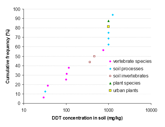
Figure 6. The species sensitivity distribution (plotted as a cumulative frequency of the toxicity data against DDT soil concentration) of soil invertebrate species, soil processes, plant species and terrestrial vertebrate species to DDT.
All the available DDT toxicity data was reported as total concentrations without making a distinction between added and background concentrations. There was no equation available able to estimate the background concentration of DDT. DDT only occurs due to its synthesis by humans. There is therefore no natural background concentration of DDT. However, due to its persistence and its ability to volatilise, DDT can be subject to long-distance transport. In fact, a global distillation hypothesis was developed and has widely been accepted as the explanation of the presence of DDT and its metabolites and other persistent organic pollutants in polar ecosystems, which have no nearby industrial point sources or non-point sources. Because of this global transport of DDT, it could be argued that there is an ABC. As the DDT toxicity studies did not provide any estimate of the ABC for DDT either at the sites or in the soils that were used, this could not be accounted for in deriving the limits for DDT. Therefore, a default ABC for DDT of 0 mg/kg was adopted.
The situation for DDT was that:
Therefore, a single value was generated by BurrliOZ (Campbell et al. 2000) for each of the three land uses. The output was the SQG(NOEC & EC10) for each particular land use and no soil-specific SQGs could be calculated. As DDT biomagnifies, the SQGs must take this into account. The methodology for deriving SQGs (Schedule B5b) for biomagnifying contaminants is to increase the level of protection (% of species to be protected) by 5% for soils for urban residential/public open space and commercial/industrial land uses to 85% and 65% of species respectively. For areas of ecological significance land uses no increase in the level of protection is recommended (Schedule B5b) as the default level (that is, for non-biomagnifying contaminants) is already 99% protective of species. The methodology was adopted and the resulting SQG(NOEC & EC10) values are presented in Table 43.
Table 43. Soil quality guidelines based on no observed effect concentration and 10% effect concentration toxicity data (SQG(NOEC & EC10)) for DDT in freshly contaminated soils with different land uses.
Land use | SQG(NOEC & EC10) (mg total DDT/kg soil) |
Areas of ecological significance | 1a |
Urban residential/public open space | 70b |
Commercial/industrial | 250c |
a to protect 99% of species, b to protect 85% of species, c to protect 65% of species.
It should be noted that if a site-specific ABC for DDT is determined (and there is sufficient justification for this ABC to be used instead of the default value of 0 mg/kg) then it may be added to the above generic SQG(NOEC & EC10) values to obtain a site-specific SQG(NOEC & EC10). As the values in Table 43 are generic SQG(NOEC & EC10) values they should be applied to all Australian soils that have the particular land use.
The SQG(LOEC & EC30) and SQG(EC50) values were calculated using the same method as that for the corresponding values for Zn, As and naphthalene. The data used to calculate these SQGs is presented in Table 42. To maximise the data available to generate the SQG(LOEC & EC30) and SQG(EC50) values, the available toxicity data was converted to the appropriate measure of toxicity using the default conversion factors recommended in Schedule B5b and presented in Table 30.
As with the SQG(NOEC & EC10) values for DDT, soil-specific SQG(LOEC & EC30) and SQG(EC50) values could not be generated, so rather a single generic SQG(LOEC & EC30) and SQG(EC50) was generated for each of the three land uses (Table 44). As these are generic SQGs, they should be applied to all Australian soils with the particular land use.
Table 44. Soil quality guidelines for DDT in freshly contaminated soil with different land uses based on lowest observed effect concentration and 30% effect concentration toxicity data, and based on 50% effect concentration toxicity data.
Land use | SQG(LOEC & EC30) (mg/kg total DDT) | SQG(EC50) (mg/kg total DDT) |
Areas of ecological significance | 3 | 6 |
Urban residential/public open space | 180 | 360 |
Commercial/industrial | 640 | 1300 |
There is currently no ageing or leaching factor available for DDT and therefore SQGs for aged contamination could not be derived.
The DDT SQGs were considered to be of moderate reliability as the toxicity data set met the minimum data requirements to use an SSD method but there were no normalisation relationships available to account for soil characteristics (Schedule B5b).
The most common metabolites of DDT are shown in Table 45. DDE is a well-known metabolite of DDT and is relatively well studied. However, there is considerably less information available on the environmental fate, metabolism, degradation and toxicity of these metabolites than on DDT. The HILs and some soil quality guidelines use a sum of DDT, DDE and DDD concentration as an SQG , for example, the Dutch and Flemish SQGs. An SQG could be derived for the sum of DDT, DDE and DDD by assuming the compounds have concentration-additive toxicity.
Table 45. Major metabolites of DDT (Sourced from WHO 1989).
Abbreviation of metabolite | Chemical name of metabolite |
DDE | 1,1'-(2,2-dichloroethenylidene)-bis[4-chlorobenzene] |
TDE(DD) | 1,1'-(2,2-dichloroethylidene)-bis[4-chlorobenzene] |
DDMU | 1,1'-(2-chloroethenyldene)-bis[4-chlorobenzene] |
DDMS | 1,1'-(2-chloroethylidene)-bis[4-chlorobenzene] |
DDNU | 1,1'-bis(4-chlorophenyl)ethlyene |
DDOH | 2,2-bis(4-chlorophenyl)ethanol |
DDA | 2,2-bis(4-chlorophenyl)-acetic acid |
Methoxychlor | 1,1'-(2,2,2-trichloroethylidene)-bis[4-methoxybenzene] |
Perthane | 1,1'-(2,2-dichloroethylidene)-bis[4-ethylbenzene] |
DFDT | 1,1'-(2,2,2-trichloroethylidene)-bis[4-fluorobenzene] |
Soil quality guidelines for DDT in a number of jurisdictions are presented in Table 46. These SQGs have a variety of purposes and levels of protection and therefore a comparison of the values is problematic. The SQGs for DDT range from 0.01 to 4 mg/kg total DDT, both from the Netherlands. The original NEPM (NEPC 1999) did not include an EIL for DDT. However, there are four HIL values of 260, 700, 400 and 4,000 mg/kg for land use settings A, B, C and D[3] for the sum of DDT, DDD, and DDE (Schedule B1). The SQGs for urban residential/public open space soil contaminated with fresh DDT based on NOEC & EC10, LOEC & EC30, and EC50 data were 70, 170 and 350 mg/kg. These values are considerably higher than the SQGs from other jurisdictions and this reflects the different methods that are used to account for biomagnification. The SQG(NOEC and EC10) and SQG(LOEC & EC30) are approximately 27% and 67% respectively, of the HIL for the standard residential setting ( setting A) which assumes direct exposure and the consumption of some food grown on the contaminated soil. The SQGs should still offer a considerable degree of protection.
Table 46. Soil quality guidelines for DDT in a number of jurisdictions.
Name of the DDT soil quality guideline | Value of the guideline (mg/kg as total) |
Dutch target values1 | 0.01 |
Dutch intervention value1 | 4 |
Canadian SQG (residential)2 | 0.7 |
Eco-SSL plants3 | NA |
Eco-SSL soil invertebrates3 | NA |
Eco-SSL avian3 | 0.093 |
Eco-SSL mammalian3 | 0.021 |
EU potentially unacceptable (residential)4 | 14 |
1 = VROM 2000
2 = CCME 1999d, 2006 and http://www.ccme.ca/publications/list_publications.html#link2
3 = http://www.epa.gov/ecotox/ecossl/
4 = Carlon 2007
NA = not available
The following compounds were considered in deriving the SQGs for Cu:
The two key considerations in determining the most important exposure pathways for inorganic contaminants are whether they biomagnify and whether they have the potential to leach to groundwater.
A surrogate measure of the potential for a contaminant to leach is its watersoil partition coefficient (Kd). If the logarithm of the Kd (log Kd) of an inorganic contaminant is less than 3, then it is considered to have the potential to leach to groundwater (Schedule B5b). The Australian National Biosolids Research Program measured the log Kd of Cu in 17 agricultural soils throughout Australia. These measurements showed that, in most soils, the log Kd of Cu was below 3 L/kg (unpublished data). The log Kd value for Cu reported by Crommentuijn et al. (2000) was 2.99 L/kg. Therefore, there is the potential for Cu in some soils to leach to groundwater and affect aquatic ecosystems. However, the methodology for SQG derivation (Schedule B5b) does not advocate the routine derivation of SQGs that account for leaching potential. Rather, it advocates that this be done on a site-specific basis as appropriate (Schedule B5b).
Copper is an essential element for the vast majority of living organisms and, as such, concentrations of Cu in tissue are highly regulated and it does not biomagnify (Louma & Rainbow 2008; Heemsbergen et al. 2008; EC 2008a). Therefore, the biomagnification route of exposure does not need to be considered for Cu and the SQGs will only account for direct toxicity.
The ecotoxicology of Cu has been extensively studied both within Australia and internationally. Most studies presented their toxicity data as an added concentration (that is, the concentration of the contaminant added to the soil that causes a specified toxic effect) or in a form that permitted the added concentration to be calculated (that is, by subtracting the background from the total concentration).
The toxicity database used to calculate the SQGs for Cu consisted of over 400 toxicity measures for 11 soil processes (Table 47), 10 invertebrate species (Table 48) and 18 plant species (Table 49). The raw data used to generate Tables 4749 is provided in Appendix E. There was sufficient data—that is, toxicity data for at least five species or soil processes that belong to at least three taxonomic or nutrient groups (Schedule B5b)—available to derive SQGs using a species sensitivity distribution (SSD) methodology.
Given that Cu does not biomagnify, the level of protection recommended in the SQG derivation methodology for urban residential/public open space land is 80% (that is, 80% of species would be protected) (Schedule B5b).
Table 47. The lowest geometric mean values of the normalised copper (Cu) toxicity data (expressed in terms of added Cu) for soil microbial processes.
Soil process | Geometric means (mg/kg added Cu) | ||
| EC10 or NOEC | EC30 or LOEC | EC50 |
Ammonification | 721 | 1081 | 2164 |
Denitrification | 59.6 | 149 | 179 |
Glutamic acid decomposition | 64.7 | 329 | 659 |
Maize residue mineralisation | 199 | 299 | 597 |
Microbial biomass carbon | 35.6 | 80.9 | 107 |
Microbial biomass nitrogen | 141 | 90.9 | 174 |
N mineralisation | 81 | 84 | 160 |
Potential nitrification rate | 137 | 205 | 282 |
Respiration | 151 | 916 | 3165 |
Substrate induced nitrification | 276 | 421 | 700 |
Substrate induced respiration | 86 | 224 | 589 |
Table 48. The lowest geometric mean values of the normalised copper (Cu) toxicity data (expressed in terms of added Cu) for soil invertebrate species.
Species | Geometric means (mg/kg added Cu) | |||
Common name | Scientific name | EC10 or NOEC | EC30 or LOEC | EC50 |
Earthworm | Eisenia andrei | 44.3 | 66.5 | 133 |
Earthworm | Eisenia fetida | 61.4 | 129 | 169 |
Earthworm | Lumbriculus rubellus | 42.4 | 117 | 656 |
Mite | Hypoapsis aculeifer | 195 | 293 | 586 |
Mite | Platynothrus peltifer | 70.7 | 106 | 212 |
Nematode | Plectus acuminatus | 27.6 | 86.4 | 259 |
Potworm | Cognettia sphagnetorum | 36.2 | 61.7 | 94.6 |
Springtail | Folsomia fimetaria | 265 | 398 | 630 |
Springtail | Folsomia candida | 205 | 343 | 499 |
Springtail | Isotoma viridis | 135 | 202 | 405 |
Table 49. The lowest geometric mean values of the normalised copper (Cu) toxicity data (expressed in terms of added Cu) for individual plant species.
Plant species | Geometric means (mg/kg added Cu) | |||
Common name | Scientific name | EC10 or NOEC | EC30 or LOEC | EC50 |
Annual meadow grass | Poa annua | 99.4 | 90.2 | 140 |
Barley | Hordeum vulgare | 47.5 | 74.6 | 187 |
Canola | Brassica napus | 825 | 1157 | 1125 |
Cotton | Gossypium sp. |
|
|
|
Groundsel | Senico vulgaris | 27.8 | 56.4 | 87.7 |
Maize | Zea mays |
|
|
|
Millet | Panicum milaceum |
|
|
|
Oats | Avena sativa | 147 | 221 | 442 |
Peanuts | Arachis hypogaea |
|
|
|
Perennial ryegrass | Lolium perenne | 69.5 | 374 | 690 |
Smooth hawkesbeard | Hypochoeris radicata | 98.2 | 164 | 186 |
Sorghum | Sorghum sp. |
|
|
|
Sugar cane | Sacharum sp. |
|
|
|
Tomato | Lycopersicon esculentum | 126 | 196 | 325 |
Triticale | Tritosecale sp. |
|
|
|
Wheat | Triticum aestivum |
|
|
|
Wild buckwheat | Polygonum convolvulus | 124 | 196 | 169 |
Daisy family | Andryala integrifolia | 75.5 | 105 | 127 |
A normalisation relationship is an empirical model that predicts the toxicity of a single contaminant to a single species using soil physicochemical properties (for example, soil pH and organic carbon content). Normalisation relationships are used to account for the effect of soil characteristics on toxicity data. Thus, when toxicity data is normalised the effect of soil properties on the toxicity should be removed, so the resulting toxicity data should more closely reflect the inherent sensitivity of the test species.
Eighteen normalisation relationships were reported in the literature for Cu toxicity and an additional two were derived as part of this study (Table 50), giving a total of 20 normalisation relationships. Six were developed for Australian soils (Broos et al. 2007; Warne et al. 2008a; Warne et al. 2008b) and fourteen have been derived for European soils (Oorts et al. 2006a; Rooney et al. 2006; Criel et al. 2008; EC 2008a). Eight of the relationships were for plants, six for soil invertebrates, and six for microbial functions (Table 50).
The choice of normalisation relationships to be used to normalise the toxicity data was based on (1) regional relevance, (2) whether they are based on field- or laboratory-based toxicity data; preference is given to field-based relationships as they provide better estimates of toxicity in the field (Warne et al. 2008b), (3) providing a conservative SQG—normalisation relationships with lower gradients will provide lower normalised toxicity values and thus lower SQGs (EC 2008a), (4) the quality of the relationship as indicated by the coefficient of determination ( r2), and (5) the number of species to which the relationships apply.
Thus, whenever there were appropriate Australian normalisation relationships, these were applied to Australian toxicity data and the same rule applied to European normalisation relationships.
Of the Australian relationships, number 1 was not used as an equivalent field-based relationship for Australian soils was available (relationship 3) and relationship 2 was not used as ultimately it is the amount of harvestable food that is most important when considering crops. The best relationship developed by Broos et al. (2007) for substrate induced nitrification, (SIN) (relationship 4) was based on EC50 and pH. However, to be consistent with all the other normalisation relationships developed, the data was re-analysed using the logarithm of the EC50 data, which resulted in relationship 5, used in this Schedule. Relationship 7 was not used as relationships not explaining at least 60% of the variation are not considered appropriate for normalisation (Warne et al. 2008b). Relationship 3 was used to normalise all the Australian plant toxicity data and relationship 5 was used to normalise all the Australian microbial process toxicity data.
Of the European relationships, 8 rather than 7 was used for barley as it contained fewer parameters and had a marginally higher r2 value. Relationship 11 was used for tomato rather than relationships 9 and 10, as Fe oxide content of soils was not reported in the vast majority of the toxicity data and as relationship 11 had a lower gradient than relationship 10. For E. Fetida, relationship 13 was used as it had a lower gradient than relationship 12. Similarly, relationship 16 for F. candida was used rather than relationships 14 or 15 as it had a lower gradient.
All the toxicity data for European plant species, apart from barley, was normalised using relationship 11 for tomato as it was the plant relationship with the lowest gradient. All the European invertebrate toxicity data was normalised using relationship 13 for E. fetida as it was the invertebrate relationship with the lowest gradient and relationship 18 for SIR was used to normalise all European microbial process toxicity data (except that for maize residue mineralisation and potential nitrification rate) as it was the microbial process relationship with the lowest positive gradient.
All the Cu toxicity data in Tables 47–49 was normalised to its equivalent toxicity in the recommended Australian reference soil (Schedule B5b) (Table 6). Depending on the conditions under which the toxicity tests were conducted, the normalised toxicity data could be higher or lower in the reference soil compared to the original toxicity data in the test soil.
Table 50. Normalisation relationships for the toxicity of copper (Cu) to plants, soil invertebrates and soil processes. The relationships used to normalise the toxicity data are in bold.
Eqn no. | Species/soil process | Y parameter | X parameter(s) | Reference | |
Australian relationships | |||||
1 | Triticum aestivum (wheat) | log EC10a (laboratory-based data) | 0.98 log CECb – 2.97 EC + 2.01 (r2 adj = 0.79) | Warne et al. 2008a | |
2 | T. aestivum (wheat) | log EC50 (field-based 8wk growth) | 0.54 pHc – 0.16 (r2 adj = 0.85) | Warne et al. 2008b | |
3 | T. aestivum (wheat) | log EC10 (field-based grain yield) | 0.31 pHc + 1.05 log OC + 0.56 (r2 adj = 0.80) | Warne et al. 2008b | |
4 | SIN | EC50 | 434 pHc – 1615 (r2 adj = 0.73) | Broos et al. 2007 | |
5 | SIN | log EC50 | 0.35 pHc + 0.84 (r2 adj = 0.72) | This study | |
6 | SIR | EC50d | 22 clay + 641 (r2 adj = 0.38) | Broos et al. 2007 | |
Northern hemisphere relationships | |||||
7 | Hordeum vulgare (barley) | log EC10a | 0.403 log CECe + 0.42 OC + 0.809 (r2 adj = 0.63) | Rooney et al. 2006 | |
8 | H. vulgare (barley) | log EC50 | 1.06 log CECe + 1.42 | EC 2008a | |
9 | Lycopersicon esculentum (tomato) | log EC10a | 0.855 log CECe + 0.388 log Fe oxide – 0.047 (r2 adj = 0.72) | Rooney et al. 2006 | |
10 | L. esculentum (tomato) | log EC10a | 0.99 log CECe, f | EC 2008a | |
11 | L. esculentum (tomato) | log EC50 | 0.96 log CECe + 1.47 | EC 2008a | |
12 | Eisenia fetida (earthworm) | log EC10 | 0.606 log CECe + 1.56 | Criel et al. 2008 | |
13 | E. fetida (earthworm) | log EC50 | 0.58 log CECe + 1.85 | EC 2008a | |
14 | Folsomia candida (collembola) | log EC10 | 1.16 log CECe + 1.1 (r2 = 0.54) | Criel et al. 2008 | |
15 | F. candida (collembola) | log EC50 | 0.96 log CECe + 1.63 | EC 2008a | |
16 | F. candida (springtail) | Log EC10 | 0.8475 log CECe + 1.499 | This study | |
17 | F. fimetria (springtail) | Log EC10 | 0.7508 log CECe + 2.0868 (r2 = 0.63) | This study | |
18 | SIR | log EC50 | 0.66 log OC + 1.96 (r2 = 0.57) | Oorts et al. 2006a | |
19 | MRM | log EC20 | -0.26 pHc + 4.05 (r2 = 0.52) | Oorts et al. 2006a | |
20 | PNR | log EC50 | 1.06 log CECe + 1.41 | Oorts et al. 2006a | |
a = normalisation relationships were also developed for the same combination of species and endpoint but for different measures of toxicity e.g. log EC50 and NOEC and using other soil physicochemical properties.
b = these CEC measurements were made using the ammonium acetate method (Rayment & Higginson 1992).
c = pH measured in 0.01 M calcium chloride (Rayment & Higginson 1992).
d = no statistically significant normalisation relationships could be derived for EC10 and EC10 SIR data (NBRP unpublished data).
e = these CEC measurements were made using the silver thiourea method (Chhabra et al. 1975).
f = the full normalisation relationship was not provided in EC (2008a) but as only the slope of the relationship is used in the normalising, the constant is not necessary. CEC = cation exchange capacity (cmolc/kg); OC = organic carbon content (%); MRM = maize residue mineralisation; PNR = potential nitrification rate; SIN = substrate induced nitrification, SIR = substrate induced respiration.
The distribution of the sensitivity of species and microbial processes to Cu is presented in Figure 7. Toxicity data for plants, soil processes and soil invertebrates was generally evenly spread in the species sensitivity distribution (SSD); however, the invertebrates did not have the same range of highly tolerant species as the other two organism groups. Nonetheless, the overall distribution of sensitivity to Cu was similar. Therefore, all the toxicity data was used to derive the ACLs and SQGs.

Figure 7. The species sensitivity distribution (plotted as a cumulative frequency against added copper (Cu) concentration) of soil processes, soil invertebrates and plant species to Cu.
As described earlier, SQGs were derived using three sets of toxicity data—NOEC and EC10, LOEC and EC30, and EC50 data.
The NOEC and EC10 toxicity data was normalised as outlined in Heemsbergen et al. (2008). Geometric means for each toxic end point (for example, mortality, reproduction, seedling emergence) for each species were calculated and the lowest geometric mean selected to represent the sensitivity of each species/microbial process. These lowest geometric means were entered into the BurrliOZ software (Campbell et al. 2000) and ACL(NOEC & EC10) values calculated that should theoretically protect 99, 80 and 60% of species/microbial processes. The resulting ACL(NOEC and EC10) values are only applicable to the Australian reference soil (Table 6). In order to generate soil-specific ACLs the normalisation relationships were applied to the ACL(NOEC & EC10) values in the reverse manner.
A complicating factor for Cu is that there are different soil physicochemical properties (that is, CEC, pH, OC and a combination of pH and log OC) that control the toxicity of Cu depending on the species or microbial process (Table 50). However, these can be rationalised down to two factors that control the ACL, namely CEC (measured using the silver thiourea method, Chhabra et al. 1975) and pH (measured in 0.01M CaCl2, Rayment & Higginson 1992) (see Appendix F for a detailed explanation of this rationalisation). Thus, there are two sets of ACL values for each land use type (that is, a set that vary with CEC and a second set that vary with pH). To determine the ACL that applies to a site, it is simply a matter of measuring the CEC and pH of the soil, looking up the tables for the appropriate ACL and then adopting the lower of the two ACL values. In the majority of cases the pH-based ACL values will limit how much Cu can be added to a soil when the soil pH is less than or equal to 6, while the CEC-based ACL values will limit the amount of Cu that can be added to a soil when the soil pH is greater than 6.
The ACL values for areas of ecological significance, urban residential/public open space and commercial/industrial land uses are presented in Tables 51 to 53, respectively.
Table 51. Soil-specific added contaminant limits (ACLs, mg/kg) based on no observed effect concentration (NOEC) and 10% effect concentration (EC10) toxicity data for fresh copper (Cu) contamination that theoretically protect at least 99% of soil processes, soil invertebrate species and plant species in soils with a pH ranging from 4.5 to 8 and a cation exchange capacity (CEC) ranging from 5 to 60 cmolc/kg and for an area of ecological significance land use. The lower of the CEC- or the pH-derived ACLs that apply to a soil is the ACL(NOEC & EC10) to be used.
Type of ACL | CEC (cmolc/kg) | |||||
| 5 | 10 | 20 | 30 | 40 | 60 |
CEC-based ACLs | 10 | 20 | 25 | 25 | 25 | 25 |
| pH | |||||
| 4.5 | 5.5 | 6 | 6.5 | 7.5 | 8.0 |
pH-based ACLs | 7 | 15 | 20 | 30 | 65 | 90 |
Table 52. Soil-specific added contaminant limits (ACLs, mg/kg) based on no observed effect concentration (NOEC) and 10% effect concentration (EC10) toxicity data for fresh copper (Cu) contamination that theoretically protect at least 80% of soil processes, soil invertebrate species and plant species in soils with a pH ranging from 4.5 to 8 and a cation exchange capacity (CEC) ranging from 5 to 60 cmolc/kg and an urban residential/public open space land use. The lower of the CEC- or the pH-derived ACLs that apply to a soil is the ACL(NOEC & EC10) to be used.
Type of ACL | CEC (cmolc/kg) | |||||
| 5 | 10 | 20 | 30 | 40 | 60 |
CEC-based ACLs | 30 | 60 | 65 | 65 | 70 | 70 |
| pH | |||||
| 4.5 | 5.5 | 6 | 6.5 | 7.5 | 8.0 |
pH-based ACLs | 20 | 40 | 60 | 85 | 170 | 250 |
Table 53. Soil-specific added contaminant limits (ACLs, mg/kg) based on no observed effect concentration (NOEC) and 10% effect concentration (EC10) toxicity data for fresh copper (Cu) contamination that theoretically protect at least 60% of soil processes, soil invertebrate species and plant species in soils with a pH ranging from 4.5 to 8 and a cation exchange capacity (CEC) ranging from 5 to 60 cmolc/kg and a commercial/industrial land use. The lower of the CEC- or the pH-derived ACLs that apply to a soil is the ACL(NOEC & EC10) to be used.
Type of ACL | CEC (cmolc/kg) | |||||
| 5 | 10 | 20 | 30 | 40 | 60 |
CEC-based ACLs | 45 | 90 | 100 | 100 | 110 | 110 |
| pH | |||||
| 4.5 | 5.5 | 6 | 6.5 | 7.5 | 8.0 |
pH-based ACLs | 30 | 60 | 90 | 130 | 270 | 380 |
To convert ACL(NOEC & EC10) values to SQG(NOEC & EC10) values, the ambient background concentration (ABC) needs to be added to the ACL(NOEC & EC10). Three methods of determining the ABC were recommended in the methodology for deriving SQGs (Heemsbergen et al. 2008).
The preferred method is to measure the ABC at an appropriate reference site. However, where this is not possible, the methods of Olszowy et al. (1995) and Hamon et al. (2004) were recommended to predict the ABC where there has been and has not been, respectively, a history of contamination. In the Hamon et al. (2004) method, the ABC for a variety of metal contaminants, including Cu, vary with either the soil iron or manganese content. The equation to predict the ABC for Cu in soils with no history of Cu contamination (Hamon et al. 2004) is:
log Cu conc (mg/kg) = 0.612 log Fe content (%) + 0.808 (equation 7)
Examples of the ABC values predicted by this equation are presented in Table 54.
Table 54. Ambient background concentrations (ABCs) for copper (Cu) predicted using the Hamon et al. (2004) method.
Fe content (%) | Predicted Cu ABC (mg/kg) |
0.1 | 2 |
0.5 | 4 |
1 | 6 |
2 | 10 |
5 | 15 |
10 | 25 |
15 | 35 |
20 | 40 |
Predicted ABC values for Cu range from approximately 2 to 40 mg/kg in soils with iron contents between 0.1 and 20%.
To calculate an SQG(NOEC & EC10), the ABC value is added to the ACL(NOEC & EC10). Ambient background concentration values vary with soil type. Therefore it is not possible to present a single set of SQGs. Thus, two examples of SQG(NOEC & EC10) values for urban settings are presented below. These examples would be at the low and high end of the range of SQG(NOEC & EC10) values (but not the extreme values) generated for Cu in Australian soils.
Example 1 |
Site descriptors urban residential/public open space land use in a new suburb (that is, fresh Cu contamination). Soil descriptors – a sandy acidic soil (pH 5.5, CEC 10) with 1% iron content. The resulting ACL(NOEC & EC10), ABC and SQG(NOEC & EC10) values are: ACL(NOEC & EC10) CEC-based: 60 mg/kg ACL(NOEC & EC10) pH-based: 40 mg/kg ACL(NOEC & EC10): 40 mg/kg (the lower of the two ACLs that apply to this soil) ABC: 6 mg/kg SQG(NOEC & EC10): 46 mg/kg, (which would be rounded off to 45 mg/kg). |
Example 2 |
Site descriptors commercial/industrial land use in a new suburb (that is, fresh Cu contamination). Soil descriptors – an alkaline clay soil (pH 7.5, CEC 40) with a 10% iron content. The resulting ACL(NOEC & EC10), ABC and SQG(NOEC & EC10) values are: ACL(NOEC & EC10) CEC-based: 110 mg/kg ACL(NOEC & EC10) pH-based: 270 mg/kg ACL(NOEC & EC10): 110 mg/kg (the lower of the two ACLs that apply to this soil) ABC: 25 mg/kg SQG(NOEC & EC10): 135 mg/kg, which would be rounded off to 130 mg/kg. |
In addition to calculating SQG(NOEC & EC10) values, Heemsbergen et al. (2008) suggested that two other sets of SQGs could be generated using either a combination of LOEC and EC30 data or EC50 data. These SQGs are termed the SQG(LOEC & EC30) and SQG(EC50) respectively. These additional SQGs were calculated using the method described in Heemsbergen et al. (2008) except the input data for the SSD was changed to the appropriate type (Table 1). The lowest geometric means of the normalised toxicity data used to generate these SQGs are presented in Tables 4749 and the raw data can be found in Appendix E. Lowest observed effect concentration, 30% effect concentration and 50% effect concentration toxicity data was not available in all instances; therefore, to maximise the data available to calculate SQG(LOEC & EC30) and SQG(EC50) values, the available NOEC and EC10 toxicity data was converted to these measures using conversion factors as necessary. The NBRP developed experimentally derived conversion factors (cited in Heemsbergen et al. 2008) for Cu and Zn (Table 17). These conversion factors were used rather than the generic conversion factors often used to convert toxicity data. This approach is consistent with the recommendation of Heemsbergen et al. (2008). Tables 55 and 56 show the soil-specific ACL(LOEC & EC30) and ACL(EC50) values respectively, for soils with areas of ecological significance, urban residential/public open space and commercial/industrial land uses.
Table 55. Soil-specific ACLs (mg/kg) based on lowest observed effect concentration (LOEC) and 30% effect concentration (EC30) data for fresh copper (Cu) contamination that should theoretically provide the appropriate level of protection (that is, 99, 80 or 60% of species) to soil processes, soil invertebrate species and plant species in soils with a pH ranging from 4.5 to 8 and a CEC ranging from 5 to 60 cmolc/kg for various land uses. The lower of the CEC- or the pH-derived ACLs for a particular land use that apply to a soil is the ACL(LOEC & EC30) to be used.
Areas of ecological significance land use | ||||||
Type of ACL | CEC (cmolc/kg)a | |||||
| 5 | 10 | 20 | 30 | 40 | 60 |
CEC-based ACLs | 25 | 50 | 50 | 55 | 55 | 60 |
| pHb | |||||
| 4.5 | 5.5 | 6 | 6.5 | 7.5 | 8.0 |
pH-based ACLs | 15 | 30 | 50 | 70 | 140 | 200 |
Urban residential/public open space land use | ||||||
Type of ACL | CEC(cmolc/kg) | |||||
| 5 | 10 | 20 | 30 | 40 | 60 |
CEC-based ACLs | 50 | 100 | 110 | 110 | 120 | 120 |
| pH | |||||
| 4.5 | 5.5 | 6 | 6.5 | 7.5 | 8.0 |
pH-based ACLs | 30 | 70 | 100 | 140 | 290 | 420 |
Commercial/industrial land use | ||||||
Type of ACL | CEC (cmolc/kg) | |||||
| 5 | 10 | 20 | 30 | 40 | 60 |
CEC-based ACLs | 70 | 150 | 160 | 170 | 170 | 180 |
| pH | |||||
| 4.5 | 5.5 | 6 | 6.5 | 7.5 | 8.0 |
pH-based ACLs | 45 | 100 | 150 | 210 | 440 | 630 |
a = CEC was measured using the silver thiourea method (Chhabra et al. 1972).
b = pH was measured using the CaCl2 method (Rayment & Higginson 1992).
Table 56. Soil-specific ACLs (mg/kg) based on 50% effect concentration (EC50) data for fresh copper (Cu) contamination that should theoretically provide the appropriate level of protection (that is, 99, 80 or 60% of species) to soil processes, soil invertebrate species and plant species in soils with a pH ranging from 4.5 to 8 and a cation exchange capacity (CEC) ranging from 5 to 60 cmolc/kg for various land uses. The lower of the CEC- or the pH-derived ACLs for a particular land use that apply to a soil is the ACL(EC50) to be used.
Areas of ecological significance land use | ||||||
Type of ACL | CEC (cmolc/kg) | |||||
| 5 | 10 | 20 | 30 | 40 | 60 |
CEC-based ACLs | 35 | 75 | 85 | 85 | 90 | 95 |
| pH | |||||
| 4.5 | 5.5 | 6 | 6.5 | 7.5 | 8.0 |
pH-based ACLs | 25 | 50 | 75 | 110 | 230 | 320 |
Urban residential/public open space land use | ||||||
Type of ACL | CEC | |||||
| 5 | 10 | 20 | 30 | 40 | 60 |
CEC-based ACLs | 85 | 170 | 190 | 200 | 200 | 210 |
| pH | |||||
| 4.5 | 5.5 | 6 | 6.5 | 7.5 | 8.0 |
pH-based ACLs | 50 | 120 | 170 | 250 | 510 | 730 |
Commercial/industrial land use | ||||||
Type of ACL | CEC (cmolc/kg) | |||||
| 5 | 10 | 20 | 30 | 40 | 60 |
CEC-based ACLs | 125 | 260 | 280 | 290 | 310 | 320 |
| pH | |||||
| 4.5 | 5.5 | 6 | 6.5 | 7.5 | 8.0 |
pH-based ACLs | 80 | 180 | 260 | 380 | 770 | 1100 |
The ABC values were calculated using the method described earlier and the values presented in Table 54.
As the ACL and ABC values are both soil-specific it is not possible to generate a single set of SQGs. Example SQGs that represent values that at the upper and lower end of the range of values that would be encountered in urban situations are presented. Two examples are presented for SQGs based on LOEC and EC30 data and two examples based on EC50 data.
SQG(LOEC & EC30)—Example 1 |
Site descriptors urban residential/public open space land use in a new suburb. Soil descriptors – a sandy acidic soil (pH 5.5, CEC 10) with 1% iron content. The resulting ACL(LOEC & EC30), ABC and SQG(LOEC & EC30) values are: ACL(LOEC & EC30) CEC-based: 100 mg/kg ACL(LOEC & EC30) pH-based: 70 mg/kg ACL(NOEC & EC10): 70 mg/kg (the lower of the two ACLs that apply to this soil) ABC: 6 mg/kg SQG(LOEC & EC30): 76 mg/kg, which would be rounded off to 75 mg/kg. |
SQG(LOEC & EC30)—Example 2 |
Site descriptors commercial/industrial land use in a new suburb. Soil descriptors – an alkaline clay soil (pH 7.5, CEC 40) with a 10% iron content. The resulting ACL(LOEC & EC30), ABC and SQG(LOEC & EC30) values are: ACL(LOEC & EC30) CEC-based: 170 mg/kg ACL(LOEC & EC30) pH-based: 440 mg/kg ACL(NOEC & EC10): 170 mg/kg (the lower of the two ACLs that apply to this soil) ABC: 25 mg/kg SQG(LOEC & EC30): 195 mg/kg, which would be rounded off to 190 mg/kg. |
SQG(EC50)—Example 1 |
Site descriptors urban residential/public open space land use in a new suburb. Soil descriptors – a sandy acidic soil (pH 5.5, CEC 10) with 1% iron content. The resulting ACL(EC50), ABC and SQG(EC50) values are: ACL(EC50) CEC-based: 170 mg/kg ACL(EC50) pH-based: 120 mg/kg ACL(EC50): 120 mg/kg (the lower of the two ACLs that apply to this soil) ABC: 6 mg/kg SQG(EC50): 126 mg/kg ,which would be rounded off to 130 mg/kg. |
SQG(EC50) - Example 2 |
Site descriptors commercial/industrial land use in a new suburb. Soil descriptors – an alkaline clay soil (pH 7.5, CEC 40) with a 10% iron content. The resulting ACL(EC50), ABC and SQG(EC50) values are: ACL(EC50) CEC-based: 310 mg/kg ACL(EC50) pH-based: 770 mg/kg ACL(EC50): 310 mg/kg (the lower of the two ACLs that apply to this soil) ABC: 25 mg/kg SQG(EC50): 335 mg/kg ,which would be rounded off to 330 mg/kg. |
In addition to calculating SQGs in recently contaminated soils (that is, contamination is <2 years old), Heemsbergen et al. (2008) suggested that an identical set of SQGs could be derived for soils where the contamination is aged (that is, it has been present for ≥2 years). The Cu SQG(NOEC & EC10), SQG(LOEC & EC30) and SQG(EC50) values for aged sites were calculated using the methods set out in earlier sections, the only difference being that laboratory toxicity data based on freshly spiked soils or soils that had not been leached were multiplied by an ALF (Schedule B5b). An ALF of 2 was developed by Smolders et al. (2009) while a value of 2.2 was developed and used in the EC ecological risk assessment for Cu (EC 2008a). Given the uniformity of these ALF values and to err on the conservative side (that is to offer greater protection to the environment), an ALF of 2 was adopted in this study.
The raw toxicity data (Appendix E) for Cu that was generated using freshly spiked and non-leached soils was multiplied by the ALF of 2. That data that was field-based and aged and/or leached laboratory-based data was not multiplied by the ALF. In all other ways the aged ACL(NOEC & EC10) and SQG(NOEC & EC10) values were calculated using the same methods as described in earlier sections. The resulting soil-specific ACL(NOEC & EC10) values for aged Cu contamination are presented in Table 57.
Table 57. Soil-specific ACLs (mg/kg) based on no observed effect concentration (NOEC) and 10% effect concentration (EC10) data for aged copper (Cu) contamination that should theoretically provide the appropriate level of protection (i.e., 99, 80 or 60% of species) to soil processes, soil invertebrate species and plant species in soils with a pH ranging from 4.5 to 8 and a CEC ranging from 5 to 60 cmolc/kg for various land uses. The lower of the CEC- or the pH-derived ACLs for a particular land use that apply to a soil is the aged ACL(NOEC & EC10) to be used.
Areas of ecological significance land use | ||||||
Type of ACL | CEC (cmolc/kg) | |||||
| 5 | 10 | 20 | 30 | 40 | 60 |
CEC-based ACLs | 15 | 25 | 30 | 30 | 30 | 35 |
| pH | |||||
| 4.5 | 5.5 | 6 | 6.5 | 7.5 | 8.0 |
pH-based ACLs | 8 | 20 | 25 | 40 | 80 | 110 |
Urban residential/public open space land use | ||||||
Type of ACL | CEC | |||||
| 5 | 10 | 20 | 30 | 40 | 60 |
CEC-based ACLs | 50 | 110 | 110 | 120 | 120 | 130 |
| pH | |||||
| 4.5 | 5.5 | 6 | 6.5 | 7.5 | 8.0 |
pH-based ACLs | 30 | 70 | 110 | 150 | 310 | 440 |
Commercial/industrial land use | ||||||
Type of ACL | CEC (cmolc/kg) | |||||
| 5 | 10 | 20 | 30 | 40 | 60 |
CEC-based ACLs | 80 | 160 | 180 | 180 | 190 | 200 |
| pH | |||||
| 4.5 | 5.5 | 6 | 6.5 | 7.5 | 8.0 |
pH-based ACLs | 50 | 110 | 160 | 230 | 480 | 680 |
For aged contaminated sites (that is, the contamination has been in place for at least 2 years) the methodology (Schedule B5b) recommends using the 25th percentiles of the ABC data for the ‘old suburbs’ from Olszowy et al. (1995) (see Table 58).
Table 58. Copper (Cu) ambient background concentrations (ABC) based on the 25th percentiles of Cu concentrations in ‘old suburbs’ (that is, >2 years old) from various states of Australia (Olszowy et al. 1995).
Suburb type | 25th percentile of Cu ABC values (mg/kg) | |||
NSW | QLD | SA | VIC | |
Old suburb, low traffic | 20 | 10 | 15 | 10 |
Old suburb, high traffic | 30 | 15 | 25 | 10 |
SQGs are the sum of the ABC and ACL values, both of which are soil-specific. It is, therefore, not possible to present a single set of SQGs. Thus, some examples of SQG(NOEC & EC10) values for aged urban soils are provided below. These examples represent SQG(NOEC & EC10) values that would be at the low and high end of the range of SQG(NOEC & EC10) values that would be generated for Cu in Australian soils, but are not extreme values.
Example 1 |
Site descriptors – urban residential land /public open space use in an old Victorian suburb with low traffic volume. Soil descriptors – a sandy acidic soil (pH 5.5, CEC 10) with 1% iron and aged Cu contamination and a low traffic volume. The resulting aged ACL(NOEC & EC10), ABC and SQG(NOEC & EC10) values are: aged ACL(NOEC & EC10) CEC-based: 110 mg/kg aged ACL(NOEC & EC10) pH-based: 70 mg/kg aged ACL(NOEC & EC10 ): 70 mg/kg (the lower of the two ACLs that apply to this soil) aged ABC: 10 mg/kg aged SQG(NOEC & EC10): 80 mg/kg |
Example 2 |
Site descriptors – commercial/industrial land use in an old South Australian suburb with a high traffic volume. Soil descriptors – an alkaline clay soil (pH 7.5, CEC 40) with a 10% iron and aged Cu contamination. The resulting ACL(NOEC & EC10), ABC and SQG(NOEC & EC10) values are: aged ACL(NOEC & EC10) CEC-based: 190 mg/kg aged ACL(NOEC & EC10) pH-based: 480 mg/kg aged ACL(NOEC & EC10): 190 mg/kg (the lower of the two ACLs that apply to this soil) aged ABC: 25 mg/kg aged SQG(NOEC & EC10): 215 mg/kg, which would be rounded off to 210 mg/kg. |
The ACL(LOEC & EC30) and ACL(EC50) values for aged Cu contamination were calculated in the same manner as the aged ACL(NOEC & EC10) values, except that LOEC and EC30 or EC50 toxicity data was used respectively. The aged ACL(LOEC & EC30) and aged ACL(EC50) values are presented in Tables 59 and 60 respectively.
Table 59. Soil-specific added contaminant limits (ACLs, mg/kg) based on LOEC and 30% effect concentration (EC30) data for aged copper (Cu) contamination that should theoretically provide the appropriate level of protection (i.e. 99, 80 or 60% of species) to soil processes, soil invertebrate species and plant species in soils with a pH ranging from 4.5 to 8 and a CEC ranging from 5 to 60 cmolc/kg for various land uses. The lower of the CEC- or the pH-derived ACLs for a particular land use that apply to a soil is the aged ACL(LOEC & EC30) to be used.
Areas of ecological significance land use | ||||||
Type of ACL | CEC (cmolc/kg) | |||||
| 5 | 10 | 20 | 30 | 40 | 60 |
CEC-based ACLs | 30 | 65 | 70 | 70 | 75 | 80 |
| pH | |||||
| 4.5 | 5.5 | 6 | 6.5 | 7.5 | 8.0 |
pH-based ACLs | 20 | 45 | 65 | 90 | 190 | 270 |
Residential urban /public open space land use | ||||||
Type of ACL | CEC (cmolc/kg) | |||||
| 5 | 10 | 20 | 30 | 40 | 60 |
CEC-based ACLs | 95 | 190 | 210 | 220 | 220 | 230 |
| pH | |||||
| 4.5 | 5.5 | 6 | 6.5 | 7.5 | 8.0 |
pH-based ACLs | 60 | 130 | 190 | 280 | 560 | 800 |
Commercial/industrial land use | ||||||
Type of ACL | CEC (cmolc/kg) | |||||
| 5 | 10 | 20 | 30 | 40 | 60 |
CEC-based ACLs | 140 | 280 | 300 | 320 | 330 | 340 |
| pH | |||||
| 4.5 | 5.5 | 6 | 6.5 | 7.5 | 8.0 |
pH-based ACLs | 85 | 190 | 280 | 400 | 830 | 1200 |
Table 60. Soil-specific ACLs (mg/kg) based on 50% effect concentration (EC50) data for aged copper (Cu) contamination that should theoretically provide the appropriate level of protection (i.e. 99, 80 or 60% of species) to soil processes, soil invertebrate species and plant species in soils with a pH ranging from 4.5 to 8 and a CEC ranging from 5 to 60 cmolc/kg for various land uses. The lower of the CEC- or the pH-derived ACLs for a particular land use that apply to a soil is the aged ACL(EC50) to be used.
Areas of ecological significance land use | ||||||
Type of ACL | CEC (cmolc/kg) | |||||
| 5 | 10 | 20 | 30 | 40 | 60 |
CEC-based ACLs | 80 | 170 | 180 | 190 | 190 | 200 |
| pH | |||||
| 4.5 | 5.5 | 6 | 6.5 | 7.5 | 8.0 |
pH -based ACLs | 50 | 110 | 170 | 240 | 490 | 700 |
Urban residential /public open space land use | ||||||
Type of ACL | CEC (cmolc/kg) | |||||
| 5 | 10 | 20 | 30 | 40 | 60 |
CEC-based ACLs | 150 | 300 | 350 | 350 | 350 | 400 |
| pH | |||||
| 4.5 | 5.5 | 6 | 6.5 | 7.5 | 8.0 |
pH -based ACLs | 95 | 200 | 300 | 450 | 900 | 1300 |
Commercial/industrial land use | ||||||
Type of ACL | CEC (cmolc/kg) | |||||
| 5 | 10 | 20 | 30 | 40 | 60 |
CEC-based ACLs | 210 | 440 | 470 | 490 | 510 | 530 |
| pH | |||||
| 4.5 | 5.5 | 6 | 6.5 | 7.5 | 8.0 |
pH -based ACLs | 130 | 290 | 440 | 630 | 1300 | 1800 |
The ABC values for aged Cu contamination were calculated using the data from Olszowy et al. (1995), and are presented in Table 58.
Four examples of SQGs that would apply to aged Cu contamination that represent the range (but not the extremes) of SQGs that would apply to urban residential/public open space and commercial/industrial land uses are presented below.
SQG(LOEC & EC30)—Example 1 |
Site descriptors urban residential land/public open space use in an old Victorian suburb with a low traffic volume. Soil descriptors – a sandy acidic soil (pH 5.5, CEC 10) with 1% iron content. The resulting aged ACL(LOEC & EC30), ABC and SQG(LOEC & EC30) values are: aged ACL(LOEC & EC30) CEC-based: 190 mg/kg aged ACL(LOEC & EC30) pH-based: 130 mg/kg aged ACL(LOEC & EC30): 130 mg/kg (the lower of the two ACLs that apply to this soil) aged ABC: 10 mg/kg aged SQG(LOEC & EC30): 140 mg/kg |
SQG(LOEC & EC30)—Example 2 |
Site descriptors commercial/industrial land use in an old South Australian suburb with a high traffic volume. Soil descriptors – an alkaline clay soil (pH 7.5, CEC 40) with a 10% iron content. The resulting ACL(LOEC & EC30), ABC and SQG(LOEC & EC30) values are: aged ACL(LOEC & EC30) CEC-based: 330 mg/kg aged ACL(LOEC & EC30) pH-based: 830 mg/kg aged ACL(LOEC & EC30): 330 mg/kg (the lower of the two ACLs that apply to this soil) aged ABC: 25 mg/kg aged SQG(LOEC & EC30): 355 mg/kg, which would be rounded off to 350 mg/kg. |
SQG(EC50)—Example 1 |
Site descriptors urban residential land/public open space use in an old Victorian suburb with a low traffic volume. Soil descriptors – a sandy acidic soil (pH 5.5, CEC 10) with 1% iron content. The resulting ACL(EC50), ABC and SQG(EC50) values are: ACL(EC50) CEC based: 300 mg/kg ACL(EC50) pH based: 200 mg/kg ACL(EC50): 200 mg/kg (the lower of the two ACLs that apply to this soil) ABC: 10 mg/kg SQG(EC50): 210 mg/kg |
SQG(EC50)—Example 2 |
Site descriptors commercial/industrial land use in an old South Australian suburb with a high traffic volume. Soil descriptors – an alkaline clay soil (pH 7.5, CEC 40) with a 10% iron content. The resulting ACL(EC50), ABC and SQG(EC50) values are: ACL(EC50) CEC based: 510 mg/kg ACL(EC50) pH based: 1300 mg/kg ACL(EC50): 510 mg/kg (the lower of the two ACLs that apply to this soil) ABC: 25 mg/kg SQG(EC50): 535 mg/kg, which would be rounded off to 530 mg/kg. |
Based on the criteria established in the methodology for SQG derivation (Schedule B5b), all the Cu SQGs were considered to be of high reliability. This resulted as the toxicity data set easily met the minimum data requirements to use the SSD method and there were normalisation relationships available to account for soil characteristics.
A compilation of SQGs for Cu from a number of jurisdictions is presented in Table 61. These SQGs have a variety of purposes and levels of protection and therefore comparison of the SQGs amongst each other and with the Cu SQGs is problematic. As well, the vast majority of the international SQGs are not soil-specific nor do they account for ageing and leaching. One would therefore expect that the ACLs could be higher than other internationals SQGs. The international guidelines for Cu range from 14 to 1,000 mg/kg (added or total Cu) both being from member countries of the European Union (Carlon 2007). The superseded interim urban EIL (NEPC 1999) for Cu was 100 mg/kg total Cu and therefore in the middle of the range of the international Cu guidelines.
Overall, the superseded interim urban EIL lies in the lower to middle part of the range of ACLs for fresh Cu contamination, while the superseded interim urban EIL lies at the lower third of the range of ACLs for aged contamination.
All of the soil-specific ACL values for urban residential land/public open space land use (irrespective of the toxicity data on which they were based) fell within the range of the international residential SQGs, the one exception being the ACLs based on EC50 for soils where the Cu has low bioavailability (that is, high pH and high CEC), which were greater than 1,000 mg/kg added Cu.
However, this was a CEC-based ACL and, as stated earlier, when the soil pH is greater than 6, the pH-based ACLs will limit the amount of Cu that can be present in soil. When this was taken into account, all the soil-specific ACL values for residential land use fell within the range of international SQGs.
Similarly, all the ACLs for commercial/industrial land use, with the exception of the aged ACLs based on EC50, fell within the range of international SQGs for Cu. The one exception was the ACL(EC50) value that would permit concentrations nearly twice (that is, 1,800 mg/kg added) that of the collated international limits (1,000 mg/kg). However, in soils with a pH above 6, the pH-based ACL will limit the amount of Cu that is permitted in soil and thus all the ACLs for commercial/industrial land use fell within the range of international SQGs.
The Cu ACL(NOEC & EC10) values in freshly contaminated urban residential/public open space soils (which should theoretically protect 80% of species) ranged from 20 to 250 mg/kg (added Cu) (Table 53). The most suitable comparison with these values is with the limits recommended by the EC Cu ecological risk assessment which used NOEC and EC10 data and should theoretically protect 95% of species. These values range from 20 to 173 mg/kg added Cu. The limits derived by these two processes are very similar.
Table 61. Soil quality guidelines for copper (Cu) from international jurisdictions.
Name of Cu limit | Numerical value of the limit (mg/kg) |
Dutch target value1 | 36 (added Cu) |
Dutch intervention level1 | 190 (added Cu) |
Canadian SQG (residential)2 | 63 (total Cu) |
Canadian SQG (commercial and industrial)2 | 91 (total Cu) |
Eco-SSL plants3 | 70 (total Cu) |
Eco-SSL soil invertebrates3 | 80 (total Cu) |
Eco-SSL avian3 | 28 (total Cu) |
Eco-SSL mammalian3 | 49 (total Cu) |
EU minimal risk values (residential)4 | 1470 (added and total Cu) |
EU warning risk values (residential)4 | 100500 (added and total Cu) |
EU potential risk values (residential)4 | 1001000 (added and total Cu) |
EU Cu ecological risk assessment5 | 26176 (added Cu) |
1 = VROM 2000
2 = CCME 1999e, & 2006 and http://ceqg-rcqe.ccme.ca/
3 = http://www.epa.gov/ecotox/ecossl/
4 = Carlon 2007
5 = EC 2008a.
The following compounds were considered in deriving the SQGs for lead (Pb):
If the logarithm of the Kd (log Kd) of an inorganic contaminant is less than 3 then it is considered to have the potential to leach to groundwater (Schedule B5b). The log Kd reported by Commentuijn et al. (2000) for Pb was 3.28 L/kg so there is little potential for Pb to leach to groundwater. If this exposure pathway were considered important at a site, then the methodology for SQG derivation advocates that this be addressed on a site-specific basis as appropriate (Schedule B5b).
The bioconcentration, bioaccumulation and biomagnification of Pb in aquatic ecosystems have received considerable attention. There has also been considerable attention paid to bioconcentration in terrestrial ecosystems but the biomagnification work has been more limited and often restricted to only examining transfer from food to consumer and not subsequent steps up food chains. One hundred and one terrestrial bioaccumulation factor (BAF) values for Pb have been published (LDA 2008) and these range from 0.00 to 6.86 with a median value of 0.1 kgdw/kgww (where dw = dry weight and ww = wet weight). The EU ecological risk assessment for Pb (LDA 2008) followed the EU technical guidance document (EC 1996), which applies assessment factors to the lowest NOEC for oral exposure of birds and mammals to account for the potential of Pb to biomagnify. However, using this method led to the derivation of limits that were below the concentrations found in control foods (that is, food that would occur in soils with background concentrations of Pb). These limits therefore imply that food (animal or plant) grown in soils with background concentrations poses a risk, which is not consistent with real-world experience. They therefore used an SSD method to determine the predicted no-effect concentration (PNEC) for oral exposure of birds and mammals and obtained a soil limit of 491 mg/kg. This value was higher than the limit based on direct exposure of soil organisms of 333 mg/kg.
Thus, it is apparent that Pb does not pose a biomagnification risk to terrestrial ecosystems. This finding is consistent with the findings for aquatic ecosystems that Pb does not biomagnify (Eisler 1988; Suedel et al. 1994; Demayo et al. 1982; Vighi 1981; Lu et al. 1975; Henney et al. 1991) and is the conclusion reached by the EU Pb ecological risk assessment (LDA 2008). Therefore, only direct toxic effects to soil organisms were considered in the derivation of the SQGs.
All the available Pb toxicity data was reported with both the total concentration and ambient background concentration, therefore the data could be converted to added concentrations. A total of ninety-six toxicity measures were available for Pb. These were for eight plant species, five species of soil invertebrates and six microbial processes (Table 62). Thus, this met the minimum data requirements recommended by Heemsbergen et al. (2008) to use the BurrliOZ SSD method (Campbell et al. 2000). Table 62 shows the geometric means of toxicity values of each species or soil microbial process that were used to derive the SQGs for Pb. The raw toxicity data used to generate the species geometric means is presented in Appendix G. In the vaxt majority of cases the geometric means of the toxicity data increase from NOEC or EC10 to LOEC or EC30 to EC50 values. However, for F. candida, Raphanus sativa, A. sativa, P. tedea and L. Sativa, the EC50 values were lower than the LOEC and EC30 data. This reflects the fact that the Pb toxicity data was not normalised for soil properties and the toxicity tests were conducted in soils with a variety of physicochemical properties.
In order to maximise the use of the available toxicity data, conversion factors recommended in Schedule B5b to permit the inter-conversion of NOEC, LOEC, EC50, EC30 and EC10 data were used (Table 17).
Table 62. Geometric means of the toxicity of lead (Pb) (expressed in terms of added Pb) to soil invertebrates, plants and soil microbial processes.
Test species | Geometric mean (mg/kg) | |||
Common name | Scientific name | NOEC or EC10 | LOEC or EC30 | EC50 |
Invertebrates | ||||
Earthworm | Dendrobaena rubida | 129 | 194 | 387 |
Earthworm | Eisenia andrei | - | 1500 | 3410 |
Earthworm | E. fetida | 761 | 2026 | 3829 |
Earthworm | L. rubellus | 1000 | 1500 | 3000 |
Springtail | F. candida | 1797 | 3749 | 1866 |
Microbial processes | ||||
Soil process | ATP | - | - | 3018 |
Soil process | Denitrification | 250 | 500 | 750 |
Soil process | Nitrification | 337 | 505 | 1010 |
Soil process | N-mineralisation | 447 | 1095 | 1342 |
Soil process | Respiration | 655 | 982 | 1964 |
Soil process | Substrate induced respiration | 1733 | 2600 | 5200 |
Plants | ||||
Radish | Raphanus sativus | 100 | 500 | 300 |
Oat | A. sativa | 100 | 500 | 300 |
Barley | H. vulgare | 50 | 250 | 1270 |
Red spruce | Picea rubens | 141 | 212 | 1228 |
Loblolly pine | Pinus taeda | 546 | 819 | 659 |
Lettuce | Latuca sativa | 125 | 188 | 174 |
Wheat | T. aestivum | 250 | 500 | 750 |
Maize | Z. mays | 100 | 150 | 300 |
Only two normalisation relationships have been developed for Pb. One models the uptake of Pb by spring wheat (T. aesitivum) (Nan et al. 2002) while the other models Pb toxicity to lettuce (L. sativa) (Hamon et al. 2003). The toxicity normalisation relationship is presented below:
EC50 = 23 pH + 171 clay content (%) - 40 (r2 = 0.84) (equation 8)
However, while the above relationship is based on ten toxicity data sets, they were only tested in five soils. This, combined with the fact that the relationship was not validated, severely limits its applicability. The EU ecological risk assessment for Pb (LDA 2008) stated that there is no relationship between soil pH and Pb toxicity. However, it did not make any statement on whether there are relationships between Pb toxicity and other soil physicochemical properties. This was examined as part of this body of work. Relationships between the logarithm of NOEC and/or EC10 data and soil pH, log organic matter content (%), log organic carbon content (%), log clay content (%) and log cation exchange capacity (CEC) for all toxicity data combined, for plants only, for invertebrates only and for soil microbial processes only were determined (data not shown). Normalisation relationships were only derived using NOEC and EC10 data as there was considerably more of this data than LOEC and EC30 or EC50 data. Only the relationship between logarithm of Pb toxicity to plants and the logarithm of the organic carbon content was able to explain more than 50% of the variation in toxicity data (r2 = 0.56).
Normalisation relationships that explain such a low percentage of the variation (that is, <60%) are not usually used to normalise toxicity data as they do not account for enough of the variability caused by the soil (Warne et al. 2008b). The majority of the relationships derived explained less than 10% of the variation in toxicity data and only three could explain more than 10%. Thus there are no useful normalisation relationships available for Pb, so the toxicity data was not normalised to the Australian reference soil, nor were soil-specific SQGs derived.
The SSD for the Pb NOEC toxicity data is presented in Figure 8. There was only toxicity data for 19 different species/microbial processes and the available data has not been normalised; therefore, the distribution reflects the variability in sensitivity of the organisms and the effect of soil properties. There was insufficient data to make a robust assessment of the relative sensitivity of the groups of organisms. However, the distributions of all three types of organisms overlap, so it was considered appropriate to use all the toxicity data to derive the SQGs.
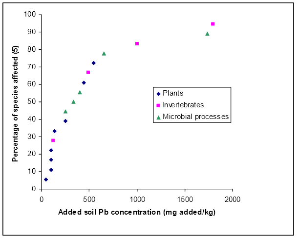
Figure 8. The species sensitivity distribution of fresh lead (Pb) contamination (plotted as a cumulative frequency of the Pb NOEC toxicity data against soil Pb concentration) for soil invertebrates, plants and microbial processes.
There was NOEC and EC10, LOEC and EC30, and EC50 Pb toxicity data so ACLs and SQGs could be derived using each of these datasets. These were generated using the same general methods as for Cu.
There were no normalisation relationships available for Pb and therefore the NOEC and EC10 toxicity data was not normalised, nor could soil-specific ACL values be derived. The single numerical output from the SSD analysis for each land use became the generic (not soil-specific) ACL for that land use and these are presented in Table 63.
Table 63. Generic ACL (mg/kg) values based on NOEC and 10% effect concentration toxicity data (EC10) for fresh lead (Pb) contamination in soil with various land uses.
Land use | ACL(NOEC & EC10) (mg/kg) |
Areas of ecological significance | 40 |
Urban residential/public open space | 130 |
Commercial/industrial | 220 |
For sites with no history of contamination, the method of Hamon et al. (2004) is recommended to estimate the ABC. The equation to predict the Pb ABC is
log Pb conc (mg/kg) = 1.039 log Fe content (%) + 0.118 (equation 9)
Examples of the ABC values predicted by this equation are presented in Table 64. Predicted ABC values for Pb range from approximately 0.1 to 30 mg/kg in soils with iron concentrations between 0.1 and 20%.
Table 64. Lead (Pb) ABCs predicted using the method of Hamon et al. (2004) (see equation 9 above).
Fe content (%) | Predicted ABC (mg/kg) |
0.1 | 0.1 |
0.5 | 0.6 |
1 | 1 |
2 | 3 |
5 | 7 |
10 | 15 |
15 | 20 |
20 | 30 |
The ABC values for Pb vary with the iron content of the soil. Therefore, it is not possible to present a specific set of SQGs(NOEC & EC10), but rather two examples of the range of SQGs that will be encountered in urban settings are presented.
Example 1 |
Site descriptors urban residential land/public open space use in a new suburb (i.e. fresh contamination). Soil descriptors – a sandy acidic soil (pH 5, CEC 10) with 1% iron content. The resulting ACL(NOEC & EC10), ABC and SQG(NOEC & EC10) values are: ACL(NOEC & EC10): 130 mg/kg ABC: 1 mg/kg SQG(NOEC & EC10): 131 mg/kg, which would be rounded off to 130 mg/kg. |
Example 2 |
Site descriptors commercial/industrial land use in a new suburb. Soil descriptors – an alkaline clay soil (pH 7.5, CEC 40) with 10% iron content. The resulting ACL(NOEC & EC10), ABC and SQG(NOEC & EC10) values are: ACL(NOEC & EC10): 220 mg/kg ABC: 15 mg/kg SQG(NOEC & EC10): 235 mg/kg, which would be rounded off to 230 mg/kg. |
ACLs based on LOEC and EC30 toxicity data (ACL(LOEC & EC30)) and based on EC50 data (ACL(EC50)) were calculated using the method used to derive the ACL values based on NOEC and EC10 data, the one exception being that in order to maximise the amount of LOEC and EC30 and EC50 data, actual measured NOEC data was used to estimate LOEC, EC30 and EC50 data. This was done using the conversion factors derived by Heemsbergen et al. (2008) and presented in Table 17. The geometric means of the LOEC and EC30 data and of the EC50 data for the various species/microbial processes that were used to derive the ACL(LOEC & EC30) and ACL(EC50) are presented in Table 62.
The resulting ACL(LOEC & EC30) and ACL(EC50) values for the three land uses are presented in Table 65. As expected, these values are larger than the corresponding ACL(NOEC & EC10) values. The ACL(EC50) values are also generally larger than the ACL(LOEC & EC30) values, with the exception of the values for areas of ecological significance. This occurs because the slope of the SSD for the LOEC and EC30 data is less than that of the EC50 data, the SSDs intersect and the LOEC and EC30 data ends up having larger toxicity values.
Table 65. Generic ACLs (mg/kg) based on LOEC and 30% effect concentration data (EC30) and based on 50% effect concentration data (EC50) values for fresh lead (Pb) contamination in soil with various land uses.
Land use | ACL(LOEC & EC30) (mg/kg) | ACL(EC50) (mg/kg) |
Areas of ecological significance | 110 | 60 |
Urban residential/public open space | 270 | 490 |
Commercial/industrial | 440 | 890 |
The ABC values for Pb were calculated using the Hamon et al. (2004) method as outlined previously.
As stated previously, the ABC values for Pb vary with the iron content of the soil. Therefore it is not possible to present a specific set of SQG (LOEC & EC30) or SQG (EC50) values. Four examples of SQGs that would apply to aged Pb contamination that represent the range (but not the extremes) of SQGs that would apply to urban residential/public open space and commercial/industrial land uses are presented below.
SQG(LOEC & EC30) Example 1 |
Site descriptors urban residential land/public open space use in a new suburb (that is, fresh contamination). Soil descriptors – a sandy acidic soil (pH 5, CEC 10) with 1% iron content. The resulting ACL(LOEC & EC30), ABC and SQG(LOEC & EC30) values are: ACL(LOEC & EC30): 270 mg/kg ABC: 1 mg/kg SQG(LOEC & EC30): 271 mg/kg, which would be rounded off to 270 mg/kg. |
SQG(LOEC & EC30) Example 2 |
Site descriptors commercial/industrial land use in a new suburb. Soil descriptors – an alkaline clay soil (pH 7.5, CEC 40) with 10% iron content. The resulting ACL(LOEC & EC30), ABC and SQG(LOEC & EC30) values are: ACL(LOEC & EC30): 440 mg/kg ABC: 15 mg/kg SQG(LOEC & EC30): 455 mg/kg, which would be rounded off to 450 mg/kg. |
SQG(EC50) Example 1 |
Site descriptors urban residential land/public open space use in a new suburb (that is, fresh contamination). Soil descriptors – a sandy acidic soil (pH 5, CEC 10) with 1% iron content. The resulting ACL(EC50), ABC and SQG(EC50) values are: ACL(EC50): 490 mg/kg ABC: 1 mg/kg SQG(EC50): 491 mg/kg, which would be rounded off to 490 mg/kg. |
SQG(EC50) Example 2 |
Site descriptors commercial/industrial land use in a new suburb. Soil descriptors – an alkaline clay soil (pH 7.5, CEC 40) with 10% iron content. The resulting ACL(EC50), ABC and SQG(EC50) values are: ACL(EC50): 890 mg/kg ABC: 15 mg/kg SQG(EC50): 905 mg/kg, which would be rounded off to 900 mg/kg. |
Smolders et al. (2009) examined the literature and developed ALFs for Pb for a range of different organisms. The resulting ALFs ranged from 1.1 to 43 with a median of 4.2. The value of 4.2, recommended by Smolders et al. (2009), was adopted and used in the EU ecological risk assessment of Pb (LDA 2008). Leaching factors for Pb have been developed for five Australian soils from South Australia, which ranged from 0.92 to 2.98 and a median and geometric mean of 1.66 and 1.61 respectively (Stevens et al. 2003).
Given the values of Stevens et al. (2003) only account for leaching and not ageing, it is likely any ALFs for Australian soils would be larger and therefore are likely to be consistent with the ALF of Smolders et al. (2009). An ALF of 4.2 was adopted in this project to calculate the SQGs for aged Pb contamination.
The ACL values for aged contamination were calculated in exactly the same manner as those for fresh contamination except that the NOEC and EC10 toxicity data was corrected using the Smolders et al. (2009) ALF of 4.2. The resulting ACL values are presented in Table 66.
Table 66. Generic ACLs (mg/kg) based on NOEC data and 10% effect concentration data (EC10) for aged lead (Pb) contamination in soil with various land uses.
Land use | ACL(NOEC & EC10) (mg/kg) |
Areas of ecological significance | 170 |
Urban residential/public open space | 530 |
Commercial/industrial | 940 |
For aged contaminated sites (that is, the contamination has been in place for at least 2 years), the methodology (Schedule B5b) recommends using the 25th percentiles of the ABC data for the ‘old suburbs’ from Olszowy et al. (1995) (see Table 67).
Table 67: Lead (Pb) ABCs based on the 25th percentiles of Pb concentrations in ‘old suburbs’ (i.e. >2 years old) from various states of Australia (Olszowy et al. 1995).
Suburb type | 25th percentile of Pb ABC values (mg/kg) | |||
NSW | QLD | SA | VIC | |
Old suburb, low traffic | 100 | 30 | 30 | 35 |
Old suburb, high traffic | 160 | 150 | 90 | 70 |
As the ABC values for Pb vary with the geographical location of the site it is not possible to present a single set of SQG(NOEC & EC10) values. Instead, two examples of the range of SQGs that will be encountered in urban settings are presented below.
Example 1 |
Site descriptors urban residential land/public open space use in an old South Australian suburb (that is, contamination is >2 years old), with low traffic volume. Soil descriptors – these are not relevant as soil properties are not considered in determining the ACL for Pb. The resulting ACL(NOEC & EC10), ABC and SQG(NOEC & EC10) values are: ACL(NOEC & EC10): 530 mg/kg ABC: 30 mg/kg SQG(NOEC & EC10): 560 mg/kg |
Example 2 |
Site descriptors commercial/industrial land use in an old Queensland suburb (that is, contamination is >2 years old), with high traffic volume. Soil descriptors – these are not relevant as soil properties are not considered in determining the ACL for Pb. The resulting ACL(NOEC & EC10), ABC and SQG(NOEC & EC10) values are: ACL(NOEC & EC10): 940 mg/kg ABC: 150 mg/kg SQG(NOEC & EC10): 1090 mg/kg, which would be rounded off to 1100 mg/kg. |
The ACL(LOEC & EC30) and ACL(EC50) values for aged Pb contamination were calculated using the method explained earlier, except that the data was multiplied by an ALF of 4.2 (Smolders et al. 2009). The resulting ACL(LOEC & EC30) and ACL(EC50) values for aged Pb contamination in the three land uses are presented in Table 68. As expected, these values are larger than the corresponding ACLs for fresh Pb contamination (Table 65).
Table 68: Generic ACLs based on LOEC and 30% effect concentration (EC30) toxicity data and based on 50% effect concentration toxicity data (EC50) values for aged lead (Pb) contamination in soil with various land uses.
Land use | ACL(LOEC & EC30) (mg/kg) | ACL(EC50) (mg/kg) |
Areas of ecological significance | 470 | 250 |
Urban residential/public open space | 1100 | 2000 |
Commercial/industrial | 1800 | 3700 |
The ABC values for aged Pb contamination were calculated using the method described earlier in this Schedule.
Four examples of SQGs that would apply to aged Pb contamination that represent the range (but not the extremes) of SQGs that would apply to urban residential/public open space and commercial/industrial land uses are presented below.
SQG(LOEC & EC30) Example 1 |
Site descriptors urban residential land/public open space use in an old South Australian (that is, contamination is >2 years old), with low traffic volume. Soil descriptors these are not relevant as soil properties are not considered in determining the ACL for Pb. The resulting ACL(LOEC & EC30), ABC and SQG(LOEC & EC30) values are: ACL(LOEC & EC30): 1100 mg/kg ABC: 150 mg/kg SQG(LOEC & EC30): 1250 mg/kg, which would be rounded off to 1,200 mg/kg. |
SQG(LOEC & EC30) Example 2 |
Site descriptors commercial/industrial land use in an old Queensland suburb (that is, contamination is >2 years old), with high traffic volume.. Soil descriptors these are not relevant as soil properties are not considered in determining the ACL for Pb. The resulting ACL(LOEC & EC30), ABC and SQG(LOEC & EC30) values are: ACL(LOEC & EC30): 1800 mg/kg ABC: 150 mg/kg SQG(LOEC & EC30): 1950 mg/kg, which would be rounded off to 1900 mg/kg, |
SQG(EC50) Example 1 |
Site descriptors urban residential land/public open space use in an old South Australian (that is, contamination is >2 years old), with low traffic volume. Soil descriptors these are not relevant as soil properties are not considered in determining the ACL for Pb. The resulting ACL(EC50), ABC and SQG(EC50) values are: ACL(EC50): 2000 mg/kg ABC: 30 mg/kg SQG(EC50): 2030 mg/kg, which would be rounded off to 2000 mg/kg. |
SQG(EC50) Example 2 |
Site descriptors commercial/industrial land use in an old Queensland suburb (that is, contamination is >2 years old), with high traffic volume. Soil descriptors these are not relevant as soil properties are not considered in determining the ACL for Pb. The resulting ACL(EC50), ABC and SQG(EC50) values are: ACL(EC50): 3700 mg/kg ABC: 150 mg/kg SQG(EC50): 3850 mg/kg, which would be rounded off to 3800 mg/kg. |
The Pb toxicity data set met the minimum data requirements to use the SSD method but there were no suitable normalisation relationships available to account for soil characteristics. Based on the criteria for assessing the reliability of SQGs (Schedule B5b), this means that the Pb SQGs were considered to be of moderate reliability.
A compilation of SQGs for Pb in a number of jurisdictions is presented in Table 69. These SQGs have a variety of purposes and levels of protection and therefore comparison of the values is problematic. The superseded interim urban EIL for Pb was 600 mg/kg total.
The urban residential/public open space ACLs for fresh Pb contamination (irrespective of the type of toxicity data on which they were based) are all lower than the superceded interim urban EIL.
The aged ACL(NOEC & EC10) for urban residential land/public open space land use, at 530 mg/kg added, is lower than the superseded interim urban EIL, while the aged ACL(LOEC & EC30) and ACL(EC50) are considerably larger (1100 and 2000 mg/kg respectively). The ACL(NOEC & EC10) for fresh Pb contamination is similar to the Canadian residential SQG and the plant Eco-SSL (Table 69).
The fresh ACL(NOEC & EC10), ACL(LOEC & EC30) and ACL(EC50) for urban residential land/public open space land use correspond to the minimal, warning and potential risk values for residential land use of the EU. The fresh ACL(NOEC & EC10) is about 50% larger than the highest minimal risk SQG, but the ACL(LOEC & EC30) and ACL(EC50) lie within the range of values for the corresponding EU SQGs.
The best comparison (in terms of the way in which the SQGs were derived) with the ACLs is with the limit derived by the EU ecological risk assessment for Pb (LDA 2008), which also corrected laboratory toxicity data for ageing and leaching. The EU derived a concentration that should protect 95% of terrestrial species of 333 mg/kg added Pb (LDA 2008). If the data and method that were used here (Schedule B5b) were used to calculate the concentration that should protect 95% of species, the value would be 275 mg/kg added Pb—this is slightly more conservative than the EU value.
Table 69. Soil quality guidelines for lead (Pb) in a number of international jurisdictions.
Name of the Pb soil quality guideline | Value of the guidelines (mg/kg) |
Canadian SQG (residential)1 | 140 (total Pb) |
Canadian SQG (commercial)1 | 260 (total Pb) |
Canadian SQG (industrial)1 | 600 (total Pb) |
Eco-SSL plants3 | 120 (total Pb) |
Eco-SSL soil invertebrates3 | 1700 (total Pb) |
Eco-SSL avian3 | 11 (total Pb) |
Eco-SSL mammalian3 | 56 (total Pb) |
Netherlands (target value) | 85 (added Pb) |
Netherlands (intervention value) | 530 (added Pb) |
EU minimal risk values (residential)2 | 2585 (added Pb) |
EU warning risk values (residential)2 | 40700 (added Pb) |
EU potential risk values (residential)2 | 100700 (added Pb) |
EC Pb ecological risk assessment (aged HC5)4 | 333 (added Pb) |
1 = CCME 1999f, 2006 and http://ceqg-rcqe.ccme.ca/
2 = Carlon 2007
3 = <http://www.epa.gov/ecotox/ecossl/>
4 = LDA 2008.
The following salts were considered in deriving SQGs for nickel (Ni):
For the leaching to groundwater pathway, adsorption (Kd) is the critical parameter. If the logarithm of the Kd (log Kd) of an inorganic contaminant is less than 3 then it is considered to have the potential to leach to groundwater (Schedule B5b). The log Kd reported by Commentuijn et al. (2000) for Ni was 2.08 L/kg, therefore there is some potential for Ni to leach to groundwater. If this exposure pathway was considered important for a given site, the methodology for SQG derivation advocates that this be addressed on a site-specific basis as appropriate (Schedule B5b).
The literature assessing the potential for Ni to biomagnify is limited, particularly for terrestrial ecosystems. However, all the available literature suggests that Ni does not biomagnify (Outridge & Schuehammer 1993; Torres & Johnson 2001; Campbell et al. 2005; Muir et al. 2005; Lapointe & Couture 2006). The EU ecological risk assessment for Ni also concluded that Ni did not biomagnify (EC 2008b). Therefore only direct toxic effects were considered in deriving the SQGs for Ni.
The raw toxicity data available for Ni is presented in Appendix H. There was a total of 338 toxicity measures for Ni. There was toxicity data for 11 plants species, 6 species of invertebrates and 26 microbial processes. The lowest geometric means of the toxicity data for each species and soil process are presented in Tables 70 and 71 respectively. This data exceeded the minimum data requirements to use the BurrliOZ software (Campbell et al. 2000) that is recommended in Schedule B5b. Therefore the SSD approach was used to derive the SQGs for Ni.
Table 70. The lowest geometric mean values of the normalised nickel (Ni) toxicity data for soil invertebrate and plant species.
Test species | Geometric means (mg/kg) | |||
Common name | Scientific name | NOEC or EC10 | LOEC or EC30 | EC50 |
Invertebrates | ||||
Earthworm | E. fetida | 162 | 245 | 474 |
Earthworm | Eisenia veneta | 103 | 365 | 409 |
Earthworm | L. rubellus | 407 | 523 | 575 |
Potworm | Enchytraeus albidus | 134 | 239 | 205 |
Springtail | F. fimetaria | 210 | 315 | 631 |
Springtail | F. candida | 235 | 359 | 680 |
Plants | ||||
Alfalfa | Medicago sativa | 36.4 | 80.8 | 87.1 |
Barley | H. vulgare | 166.7 | 250 | 409 |
Fenugreek | Trigonella poenumgraceum | 68.6 | 109 | 144 |
Lettuce | L. sativa | 52.6 | 125 | 154 |
Maize | Z. mays | 49.4 | 94.8 | 127 |
Oats | A. sativa | 55.3 | 83.9 | 122 |
Onion | Allium cepa | 37.6 | 59.7 | 84.5 |
Perennial ryegrass | L. perenne | 40.9 | 50.2 | 57.1 |
Radish | R. sativus | 57.5 | 65.5 | 66.8 |
Spinach | Spinacia oleracea | 26.9 | 41.1 | 47.2 |
Tomato | L. esculentum | 94.8 | 142 | 238 |
Table 71. The lowest geometric mean values of the normalised nickel (Ni) toxicity data for soil microbial processes.
Microbial process | Geometric means (mg/kg) | ||
NOEC or EC10 | LOEC or EC30 | EC50 | |
Arylsulfatase | 784 | 1176 | 1191 |
Aspergillus clavatus (hyphal growth) | 14.9 | 45.9 | 91.0 |
Aspergillus flavus (hyphal growth) | 451 | 586 | 689 |
Aspergillus flavipes (hyphal growth) | 398 | 444 | 475 |
Aspergillus niger (hyphal growth) | 459 | 545 | 606 |
ATP content | 75.5 | 113 | 392 |
Gliocladium sp. (hyphal growth) | 230 | 560 | 1036 |
Bacillus cereus (colony count) | 327 | 1010 | 1958 |
Dehydrogenase | 6.8 | 20.8 | 85.5 |
Glucose respiration | 79.5 | 119 | 238 |
Glutamate respiration | 44.5 | 191 | 381 |
Maize residue respiration | 134 | 201 | 402 |
Nitrification | 81.3 | 122 | 244 |
N-mineralisation | 95.8 | 144 | 287 |
Nocardia rhodochrous (colony count) | 203 | 662 | 943 |
Penicillium vermiculatum (hyphal growth) | 117 | 271 | 460 |
Phosphatase | 524 | 1347 | 5715 |
Protease | 75.5 | 113 | 392 |
Proteus vulgaris (colony count) | 17.2 | 88.8 | 249 |
Respiration (CO2 release) | 102 | 2583 | 4593 |
Rhizopus stolonifer (hyphal growth) | 331 | 404 | 459 |
Rhodotorula rubra (colony count) | 283 | 837 | 1796 |
Sacharase | 75.5 | 113 | 392 |
Serratia marcescens (colony count) | 178 | 337 | 395 |
Trichoderma viride (hyphal growth) | 608 | 686 | 740 |
Urease | 222 | 332 | 879 |
Normalisation relationships relating the toxicity of Ni to three soil microbial processes (nitrification, glucose-induced respiration and maize residue mineralisation) were developed by Oorts et al. (2006b). Two normalisation relationships have also been developed for crops (tomato and barley) by Rooney et al. (2007). In addition, the EU Ni ecological risk assessment (EC 2008b) reported Ni normalisation relationships for two soil invertebrates (F. candida and E. fetida). All of these relationships were developed for both fresh and aged contamination and are presented in Table 72. No Ni normalisation relationships have been developed for Australian species and/or soils.
The normalisation relationships presented in Table 72 all model EC50 toxicity data, with the exception of the maize residue mineralisation which models EC20 data. Relationships between the logarithm of Ni NOEC and EC10 data and logarithm of CEC were developed as part of this project. Normalisation relationships were developed for (a) all organisms, (b) each group of organisms separately, and (c) each species or microbial process separately. Only CEC was used to develop the normalisation relationships as in all the published relationships for Ni the CEC was the best parameter (Oorts et al. 2006b; Rooney et al. 2007; EC 2008b). Only six normalisation relationships could explain more than 50% of the variation in the toxicity data (i.e. r2 > 0.5) and these are presented in Table 73. The majority of the normalisation relationships had r2 values of <0.1.
Normalisation relationships are available for a variety of biological end points based on both NOEC and EC10 data and on EC50 data. The relationships used to normalise the data in the current study were relationships 1, 5 and 9 from Table 72 for glucose-induced respiration, nitrification and tomato, and relationships 2, 3, 5, 6 from Table 73 for barley, all invertebrates, maize residue mineralisation and respiration. The relationships with the lowest gradients for each species were selected. The exception to this was the relationship for invertebrates. This was selected as it was based on all invertebrate species and its gradient was only marginally higher than the invertebrate relationship with the lowest gradient. For the species that did not have normalisation relationships, the relationship for the most closely related species was used, or in the case where there were relationships for several related species, the relationship with the lowest gradient was used. Thus, all plant species (apart from tomato) were normalised with the EC10 relationship for barley and all the microbial processes without a relationship were normalised with the EC10 relationship for maize residue mineralisation.
Table 72. Normalisation relationships between soil CEC and the toxicity of nickel (Ni) to a variety of soil plant and invertebrate species and soil microbial processes for both fresh and aged contamination. The relationships used to normalise the toxicity data in this project are in bold.
Eqn no. | Species/soil process | Y parameter | X parameter(s) | Reference |
Northern hemisphere relationshipsa | ||||
1 | Glucose induced respiration | log EC50 (fresh) | 0.95 log CEC + 1.51 (r2 = 0.82) | Oorts et al. 2006b |
2 | log EC50 (aged) | 1.34 log CEC + 1.38 (r2 = 0.92) | Oorts et al. 2006b | |
3 | Maize residue mineralisation | log EC20 (fresh) | 0.86 log CEC + 1.48 (r2 = 0.55) | Oorts et al. 2006b |
4 | log EC20 (aged) | 1.22 log CEC + 1.37 (r2 = 0.72) | Oorts et al. 2006b | |
5 | Nitrification | log EC50 (fresh) | 0.79 log CEC + 1.44 (r2 = 0.69) | Oorts et al. 2006b |
6 | log EC50 (aged) | 1.00 log CEC + 1.42 (r2 = 0.60) | Oorts et al. 2006b | |
7 | Barley root elongation | log EC50 (fresh) | 0.90 log CEC + 1.60 (r2 = 0.92) | Rooney et al. 2007 |
8 | log EC50 (aged) | 1.12 log CEC + 1.57 (r2 = 0.83) | Rooney et al. 2007 | |
9 | Tomato shoot yield | log EC50 (fresh) | 1.06 log CEC + 1.09 (r2 = 0.77) | Rooney et al. 2007 |
10 | log EC50 (aged) | 1.27 log CEC + 1.06 (r2 = 0.67) | Rooney et al. 2007 | |
11 | F. candida (collembola) | log EC50 (fresh) | 0.97 log CEC + 1.71 (r2 = 0.84) | EC 2008b |
12 | log EC50 (aged) | 1.17 log CEC + 1.70 (r2 = 0.71) | EC 2008b | |
13 | Eisenia. fetida (earthworm) | log EC50 (fresh) | 0.72 log CEC + 1.79 (r2 = 0.74) | EC 2008b |
14 | log EC50 (aged) | 0.95 log CEC + 1.76 (r2 = 0.72) | EC 2008b | |
a = all the CEC measurements were made using the silver thiourea method (Chhabra et al. 1975).
Table 73. The normalisation relationships for nickel (Ni) that could explain more than 50% of the variation in the NOEC and 10% effect concentration (EC10) data. The x and y parameters in each equation are the logarithms of the CEC and of the NOEC or EC10 toxicity data, respectively. The relationships used to normalise the toxicity data in this project are in bold.
Eqn no. | Species and end point | X parameter(s)a |
1 | Tomato (shoot yield) | 1.068 x + 0.908 (r2 = 0.76) |
2 | Barley (root elongation) | 0.87 x + 1.35 (r2 = 0.86) |
3 | All invertebrates (mixed endpoints) | 0.78 x + 1.51 (r2 = 0.56) |
4 | Glucose respiration | 1.42 x – 0.38 (r2 = 0.58) |
5 | Maize residue mineralisation | 0.67 x + 1.45 (r2 = 0.53) |
6 | Respiration | 2.37 x – 0.36 (r2 = 0.92) |
a = all CEC measurements were made using the silver thiourea method (Chhabra et al. 1975).
Figure 9 shows the SSD (that is, the cumulative distribution of the geometric means of normalised NOEC and EC10 toxicity values) for the species used to derive the Ni SQGs. While there is an abundance of terrestrial toxicity data for Ni, the majority of data is for microbial processes and microbial enzymes, with only small amounts of data for plants and invertebrates. There does not appear to be any difference in the sensitivity of microbial processes and both plants and invertebrates. However, the distributions of the sensitivities of the plants and invertebrates only just overlap. Nonetheless, there are no marked differences in the sensitivity of the three groups of organisms and therefore all the available toxicity data was used to derive the Ni SQGs.

Figure 9. The SSD of normalised NOEC and 10% effect concentration (EC10) toxicity data for fresh nickel (Ni) contamination against soil Ni concentration for soil invertebrates, plants and microbial processes.
Soil quality guidelines were derived using three different sets of toxicity data (that is, NOEC and EC10, LOEC and EC30, and EC50 data) as part of this study.
All the toxicity data was normalised as set out earlier. The generic ACL(NOEC & EC10) values generated for fresh Ni contamination for the three land uses are presented in Table 74.
Table 74. Generic ACLS for fresh nickel (Ni) contamination based on NOEC and 10% effect concentration (EC10) toxicity data for various land uses.
Land use | Generic added contaminant limit |
Areas of ecological significance | 6 |
Residential urban/public open space | 50 |
Commercial/industrial | 95 |
The normalisation equations were then used to calculate soil-specific ACL values at a range of CEC values. Then the lowest ACL at each CEC value was adopted as the soil-specific ACL (Table 75).
Table 75. The soil-specific ACLs (mg/kg) at a range of cation exchange capacities for fresh nickel (Ni) contamination based on NOEC and 10% effect concentration (EC10) toxicity data.
Land use | Cation exchange capacities (cmolc/kg)a | |||||
5 | 10 | 20 | 30 | 40 | 60 | |
Areas of ecological significance | 1 | 6 | 9 | 10 | 15 | 20 |
Residential urban/public open space | 10 | 50 | 80 | 110 | 130 | 170 |
Commercial/industrial | 20 | 95 | 150 | 200 | 240 | 310 |
a = all CEC measurements were made using the silver thiourea method (Chhabra et al. 1975).
For sites with no history of Ni contamination, the method of Hamon et al. (2004) is recommended in Schedule B5b to estimate the ABC. The equation to predict the ABC for Ni is
log Ni conc (mg/kg) = 0.702 log Fe content (%) + 0.834 (equation 10)
Examples of the ABC values predicted by this equation are presented in Table 76.
Table 76. ABCs for nickel (Ni) predicted using the equation from method of Hamon et al. (2004) (equation 10 above).
Fe content (%) | Predicted ABC |
0.1 | 1 |
0.5 | 4 |
1 | 7 |
2 | 10 |
5 | 20 |
10 | 35 |
15 | 45 |
20 | 55 |
Predicted ABC values for Ni range from approximately 1 to 55 mg/kg in soils with iron contents between 0.1 and 20%.
To calculate the Ni SQG(NOEC & EC10) values, the ABC value is added to the ACL(NOEC & EC10). ABC values vary with soil type. Therefore, it is not possible to present a single set of SQG(NOEC & EC10) values. Thus, two examples of Ni SQG(NOEC & EC10) values for urban contaminated soils are provided below. These examples would be at the low and high end of the range of SQG values (but not the extreme values) generated for Australian soils.
Example 1 |
Site descriptors urban residential land/public open space use in a new suburb (that is, fresh contamination). Soil descriptors a sandy acidic soil (pH 5, CEC 10) with 1% iron content. The resulting ACL(NOEC & EC10), ABC and SQG(NOEC & EC10) values are: ACL(NOEC & EC10): 50 mg/kg ABC: 7 mg/kg SQG(NOEC & EC10): 57 mg/kg, which would be rounded off to 55 mg/kg. |
Example 2 |
Site descriptors commercial/industrial land use in a new suburb. Soil descriptors an alkaline clay soil (pH 7.5, CEC 40) with 10% iron content. The resulting ACL(NOEC & EC10)ABC and SQG(NOEC & EC10) values are: ACL(NOEC & EC10): 240 mg/kg ABC: 35 mg/kg SQG(NOEC & EC10): 275 mg/kg, which would be rounded off to 270 mg/kg. |
To maximise the data available to generate the ACL(LOEC & EC30) and ACL(EC50), the available toxicity data was converted to the appropriate measure of toxicity using the conversion factors recommended in Schedule B5b and presented in Table 17. As there were normalisation equations available, soil-specific ACLs could be generated. The ACL(LOEC & EC30) and ACL(EC50) values were calculated using the same method as that for the corresponding values for Cu and Pb and are presented in Table 77.
Table 77. The soil-specific ACLs (mg/kg) at a range of cation exchange capacities for fresh nickel (Ni) contamination based on LOEC and 30% effect concentration (EC30) toxicity data, and based on 50% effect concentration (EC50) toxicity data.
Land use | Cation exchange capacities (cmolc/kg) | |||||
5 | 10 | 20 | 30 | 40 | 60 | |
| Based on LOEC and EC30 data | |||||
Areas of ecological significance | 1 | 7 | 10 | 15 | 15 | 25 |
Residential urban/public open space | 10 | 50 | 85 | 110 | 130 | 170 |
Commercial/industrial | 20 | 100 | 170 | 220 | 260 | 350 |
| Based on EC50 data | |||||
Areas of ecological significance | 5 | 25 | 40 | 55 | 65 | 90 |
Residential urban/public open space | 30 | 160 | 250 | 330 | 400 | 520 |
Commercial/industrial | 55 | 280 | 450 | 590 | 710 | 940 |
The ABC values for Ni were calculated using the method previously set out, and the values presented in Table 76.
To calculate the Ni SQG(LOEC & EC30) and the SQG(EC50) values, the ABC value is added to the corresponding ACL values. ABC values and Ni ACL values vary with soil type. Therefore it is not possible to present a single set of SQG(LOEC & EC30) or SQG(EC50) values. Thus, two examples of Ni SQG(LOEC & EC30) and two examples for Ni SQG(EC50) are provided below. These examples would be at the low and high end of the range of SQG values (but not the extreme values) generated for Australian soils.
SQG(LOEC & EC30) Example 1 |
Site descriptors urban residential land/public open space use in a new suburb (that is, fresh contamination). Soil descriptors a sandy acidic soil (pH 5, CEC 10) with 1% iron content. The resulting ACL(LOEC & EC30), ABC and SQG(LOEC & EC30) values are: ACL(LOEC & EC30): 50 mg/kg ABC: 7 mg/kg SQG(LOEC & EC30): 57 mg/kg, which would be rounded off to 55 mg/kg. |
SQG(LOEC & EC30) Example 2 |
Site descriptors commercial/industrial land use in a new suburb. Soil descriptors an alkaline clay soil (pH 7.5, CEC 40) with 10% iron content. The resulting ACL(LOEC & EC30), ABC and SQG(LOEC & EC30) values are: ACL(LOEC & EC30): 260 mg/kg ABC: 35 mg/kg SQG(LOEC & EC30): 295 mg/kg, which would be rounded off to 290 mg/kg. |
SQG(EC50) Example 1 |
Site descriptors urban residential land/public open space use in a new suburb (that is, fresh contamination). Soil descriptors a sandy acidic soil (pH 5, CEC 10) with 1% iron content. The resulting ACL(EC50), ABC and SQG(EC50) values are: ACL(EC50): 160 mg/kg ABC: 7 mg/kg SQG(EC50): 167 mg/kg, which would be rounded off to 170 mg/kg |
SQG(EC50) Example 2 |
Site descriptors commercial/industrial land use in a new suburb. Soil descriptors an alkaline clay soil (pH 7.5, CEC 40) with 10% iron content. The resulting ACL(EC50), ABC and SQG(EC50) values are: ACL(EC50): 710 mg/kg ABC: 35 mg/kg SQG(EC50): 745 mg/kg, which would be rounded off to 750 mg/kg. |
Smolders et al. (2009) state that, based on an extensive review of the literature, the ALF for Ni is a function of soil pH (measured in 0.01 M calcium chloride solution) and ranges between 1 and 3.5. Further detail on this relationship is provided in the EU ecological risk assessment report for Ni (EC 2008b). The relationship between the ALF and soil pH is:
ALF = 1 + exp(1.4(soil pH – 7.0) (equation 11)
However, using this equation indicates that the ALF will rapidly increase after a soil pH of 7.5 to values considerably higher than 3.5 (Table 78).
Table 78. ALF values for nickel (Ni) at various soil pH values. The ALF values were derived using the relationship from the European Union ecological risk assessment for Ni (EC 2008b).
Soil pH (CaCl2) | ALF |
5 | 1.07 |
6 | 1.25 |
7 | 2.00 |
7.5 | 3.01 |
8 | 5.06 |
8.5 | 9.17 |
9.0 | 17.45 |
The above ALF values were calculated after a maximum of 1.5 years ageing in the field, therefore in most ‘aged’ Australian sites the ALFs would be larger. However, there is no information available that would permit estimates of how much larger the ALFs would be and therefore the above ALF values were used to calculate the Ni SQGs.
There are two possible approaches to incorporating the relationship between ALF and soil pH into the methodology for deriving SQGs. In the first, a soil pH that is reasonably representative or protective of the majority of Australian soils is selected and the corresponding ALF is then used to calculate the aged SQGs. The resulting SQGs would be protective of all aged soils with a pH higher than the selected pH, but would not provide the same level of protection to soils with lower soil pH. Such soils would have to proceed to further desktop analysis by using the ALFpH relationship to determine the appropriate ALF for that soil and then apply that to the fresh contamination SQGs. To maximise the utility of this approach and minimise the number of sites that would require the additional analysis, the selected soil pH would have to be low, perhaps as low as 5. This would result in an ALF of 1.07 and with such a small increase in the resulting aged SQGs, it is doubtful that it would be of any real benefit.
The second approach would be to fully adopt the ALFpH relationship into the methodology for deriving SQGs, where the pH of the site would need to be determined and then the appropriate ALF calculated for the site and applied to the toxicity data to generate the aged contamination ACLs and thence the aged SQGs. While the latter is more complex, the benefits of having the most scientifically defensible ACLs and SQGs outweigh this. It is recommended that SQGs are derived by multiplying fresh (non-aged and non-leached) toxicity data by the ALF determined using the ALFpH relationship (see equation 11).
The aged SQG(NOEC & EC10) values for Ni were calculated using the same methodology as that used for the SQG(NOEC & EC10) values for fresh Ni contamination, with two exceptions. These were (i) that the ‘fresh’ toxicity data was corrected using the Ni ALFs (equation 11) and (ii) the ABCs were the 25th percentile values for old suburbs from Olszowy et al. (1995). The resulting ACL(NOEC & EC10) values for aged Ni contamination are presented in Table 79.
Table 79. The soil-specific ACLs (mg/kg) at a range of cation exchange capacities for aged nickel (Ni) contamination based on NOEC and 10% effect concentration (EC10) toxicity data.
Land use | Cation exchange capacities (cmolc/kg) | |||||
5 | 10 | 20 | 30 | 40 | 60 | |
Areas of ecological significance | 2 | 9 | 15 | 20 | 20 | 30 |
Residential urban/public open space | 15 | 85 | 140 | 180 | 220 | 290 |
Commercial/industrial | 30 | 160 | 250 | 330 | 400 | 530 |
For aged contaminated sites (that is, the contamination has been in place for at least 2 years) Heemsbergen et al. (2008) recommends using the 25th percentiles of the ABC data for ‘old suburbs’ in Olszowy et al. (1995) (see Table 80). The Olszowy et al. (1995) data is derived from soils low in geogenic Ni and, by using low ABCs, could create low SQGs in some areas with naturally high background Ni concentrations. This problem could be overcome in areas with elevated soil Ni by using measured ABC values or using the method of Hamon et al. (2004).
Table 80. Nickel (Ni) ABCs based on the 25 percentiles of Ni concentrations in ‘old suburbs’ (i.e. >2 years old) from various states of Australia (Olszowy et al. 1995).
Suburb type | 25th percentile of Ni ABC values (mg/kg) | |||
NSW | QLD | SA | VIC | |
Old suburb, low traffic | 5 | 5 | 6 | 5 |
Old suburb, high traffic | 5 | 4 | 6 | 10 |
To calculate the aged Ni SQG(NOEC & EC10) values , the ABC value is added to the ACL. Ambient background concentration values vary with soil type, region and history of exposure to contamination. Therefore, it is not possible to present a single set of SQG(NOEC & EC10) values. Thus, two examples of Ni SQG(NOEC & EC10) values are presented below. These examples would be at the low and high end of the range of SQG values (but not the extreme values) generated for Australian soils.
Example 1 |
Site descriptors urban residential land/public open space use in an old Queensland suburb (that is, aged contamination), with low traffic volume. Soil descriptors a sandy acidic soil (pH 5, CEC 10) with 1% iron content. The resulting ACL(NOEC & EC10), ABC and SQG(NOEC & EC10) values are: ACL(NOEC & EC10): 85 mg/kg ABC: 5 mg/kg SQG(NOEC & EC10): 90 mg/kg |
Example 2 |
Site descriptors commercial/industrial land use in an old Victorian suburb (that is, aged contamination), with high traffic volume. Soil descriptors an alkaline clay soil (pH 7.5, CEC 40) with 10% iron content. The resulting ACL(NOEC & EC10), ABC and SQG(NOEC & EC10) values are: ACL(NOEC & EC10): 400 mg/kg ABC: 10 mg/kg SQG(NOEC & EC10): 410 mg/kg |
Table 81. The soil-specific ACLs at a range of cation exchange capacities for aged nickel (Ni) contamination based on lowest observed effect concentration (LOEC) and 30% effect concentration (EC30) toxicity data, and based on 50% effect concentration (EC50) toxicity data.
Land use | Cation exchange capacities (cmolc/kg) | |||||
5 | 10 | 20 | 30 | 40 | 60 | |
| Based on LOEC and EC30 data | |||||
Areas of ecological significance | 5 | 30 | 45 | 60 | 70 | 95 |
Urban residential/public open space | 30 | 170 | 270 | 350 | 420 | 560 |
Commercial/industrial | 55 | 290 | 460 | 600 | 730 | 960 |
| Based on EC50 data | |||||
Areas of ecological significance | 10 | 65 | 100 | 130 | 160 | 210 |
Urban residential/public open space | 55 | 270 | 440 | 570 | 700 | 910 |
Commercial/industrial | 90 | 460 | 730 | 960 | 1200 | 1500 |
The ABC values used for aged Ni were obtained from Table 80.
Ambient background concentration values for Ni vary with soil type as do the Ni ACL values. Therefore, it is not possible to present a single set of SQG(LOEC & EC30) or SQG(EC50) values. Thus, two examples of Ni SQG(LOEC & EC30) values and two examples for Ni SQG(EC50) values are provided below. These examples would be at the low and high end of the range of SQG values (but not the extreme values) generated for Australian soils.
SQG(LOEC & EC30) Example 1 |
Site descriptors urban residential land/public open space use in an old Queensland suburb (that is, aged contamination), with high traffic volume. Soil descriptors a sandy acidic soil (pH 5, CEC 10) with 1% iron content. The resulting ACL(LOEC & EC30), ABC and SQG(LOEC & EC30) values are: ACL(LOEC & EC30): 170 mg/kg ABC: 4 mg/kg SQG(LOEC & EC30): 174 mg/kg, which would be rounded off to 170 mg/kg. |
SQG(LOEC & EC30) Example 2 |
Site descriptors commercial/industrial land use in an old Victorian suburb, with high traffic volume. Soil descriptors an alkaline clay soil (pH 7.5, CEC 40) with 10% iron content. The resulting ACL(LOEC & EC30), ABC and SQG(LOEC & EC30) values are: ACL(LOEC & EC30): 730 mg/kg ABC: 10 mg/kg SQG(LOEC & EC30): 740 mg/kg |
SQG(EC50) Example 1 |
Site descriptors urban residential land/public open space use in an old Queensland suburb (that is, aged contamination), with high traffic volume. Soil descriptors a sandy acidic soil (pH 5, CEC 10) with 1% iron content. The resulting ACL(EC50), ABC and SQG(EC50) values are: ACL(EC50): 270 mg/kg ABC: 4 mg/kg SQG(EC50): 274 mg/kg, which would be rounded off to 270 mg/kg. |
SQG(EC50) Example 2 |
Site descriptors commercial/industrial land use in an old Victorian suburb, with high traffic volume. Soil descriptors an alkaline clay soil (pH 7.5, CEC 40) with 10% iron content. The resulting ACL(EC50), ABC and SQG(EC50) values are: ACL(EC50): 1200 mg/kg ABC: 10 mg/kg SQG(EC50): 1210 mg/kg, which would be rounded off to 1200 mg/kg. |
The SQGs for Ni were considered to be of high reliability, as the toxicity data set met the minimum data requirements to use an SSD method and there were normalisation relationships available to account for soil characteristics (Schedule B5b).
Soil quality guidelines for Ni in a number of international jurisdictions are presented in Table 82. These SQGs have a variety of purposes and levels of protection and therefore a comparison of the values is problematic. The SQGs for Ni range from 24 to 500 mg/kg added and total Ni, with both of these values coming from countries within the EU. The superseded interim urban EIL for Ni (NEPC 1999) was 60 mg/kg total Ni.
There are also four health-based investigation level (HIL) values that range from 400 to 4000 mg/kg total Ni (see Schedule B1). The urban residential/public open space ACLs based on NOEC and EC10, LOEC and EC30, and EC50 data for fresh Ni contamination range from 10–170, 10–170, and 30 to 520 mg/kg added Ni respectively. These correspond to the ’minimal risk‘, ’warning risk‘ and the ’potential risk‘ values of EU member countries and the values are very similar. The urban residential/public open space ACLs based on NOEC and EC10, LOEC and EC30, and EC50 data for aged Ni contamination range from 15290, 30560, and 55910 mg/kg added Ni respectively. These limits permit higher concentrations than in any of the other jurisdictions, but this is not suprising as the other jurisdictions do not account for ageing or leaching, nor do they take into account the bioavailability in different soils.
The most meaningful comparisons can be made between the SQGs and the concentrations that would protect 95% of species based on NOEC and EC10 data that was derived in the EU ecological risk assessment for Ni (EC 2008b). These values ranged from 8.3 to 188.7 mg/kg added Ni for soils with CEC values ranging from 2.4 to 36 cmolc/kg (EC 2008b). SQGs that protected 95% of species were not derived, but rather the SQGs were derived that protect 99, 80 and 60% of species. The SQGs that aim to protect 99% of species based on NOEC and EC10 data ranged from 120 mg/kg added Ni. The SQGs that aim to protect 80% of species based on NOEC and EC10 data ranged from 10170mg/kg added Ni. These comparisons indicate that the SQGs derived in this project are slightly more conservative than the EU values, but overall the values are similar.
Table 82. Soil quality guidelines for nickel (Ni) in a number of international jurisdictions.
Name of the Ni soil quality guideline | Value of the guideline (mg/kg Ni) |
Dutch target values1 | 35 (added Ni) |
Dutch intervention value1 | 210 (added Ni) |
Canadian SQG (residential, commercial and industrial)2 | 50 (total Ni) |
Eco-SSL plants3 | 38 (total Ni) |
Eco-SSL soil invertebrates3 | 280 (total Ni) |
Eco-SSL avian3 | 210 (total Ni) |
Eco-SSL mammalian3 | 130 (total Ni) |
EU minimal risk values (residential)4 | 2460 (added & total Ni) |
EU warning risk values (residential) | 30180 (added & total Ni) |
EU potential risk values (residential)4 | 30500 (added & total Ni) |
EU Ni ecological risk assessment (conc that should protect 95% of species)5 | 8.3188.7 (added & total Ni) |
1 = VROM 2000
2 = CCME 1999g 2006 and http://ceqg-rcqe.ccme.ca/
3 = http://www.epa.gov/ecotox/ecossl/
4 = Carlon 2007
5 = EC 2008b.
Chromium occurs in a number of oxidation states: II, III, IV, V and VI. The two dominant states in soils are trivalent (III) and hexavalent (VI) Cr. The only forms of Cr (III) for which there was toxicity data were chromium chloride, chromium nitrate and chromium sulphate.
Chromium is the seventh most abundant element (McGrath & Smith 1990). It is also an essential element for humans and for some groups of organisms (Crommentuijn et al. 2000), yet the hexavalent form is generally considered to be highly toxic and a carcinogen.
The two key considerations in determining the most important exposure pathways for inorganic contaminants, such as Cr (III), are whether they biomagnify and whether they have the potential to leach to groundwater. A surrogate measure of the potential for a contaminant to leach is its watersoil partition coefficient (Kd). If the logarithm of the Kd (log Kd) of an inorganic contaminant is less than 3 then it is considered to have the potential to leach to groundwater (Schedule B5b). The log Kd reported by Commentuijn et al. (2000) for Cr (with the oxidation state not identified) was 2.04 L/kg; therefore, Cr has the potential in some soils to leach to groundwater. However, the ability of Cr to migrate from soil to either groundwater or surface water depends greatly on its oxidation state. Hexavalent Cr is highly water-soluble whereas trivalent Cr is almost insoluble in water and immobile in soil (Bartlett & James 1988; Cervantes et al. 2001). Therefore, Cr (III) is unlikely to pose an environmental risk by leaching. In addition, Cr (III) cannot cross most cells (Cervantes et al. 2001). In contrast, Cr (VI) is actively transported across cell membranes (Dreyfuss, 1964; Wiegand et al. 1985). Chromium (III) is not known to biomagnify (Scott-Fordsmand & Pedersen 1995; Heemsbergen et al. [2008]) and therefore only direct toxicity routes of exposure were considered in deriving the SQGs for Cr (III).
Unlike the preceding elements, there is a lack of ecotoxicity data for Cr (III). This is reflected by the fact that the US EPA (US EPA 2008) could not derive Eco-SSL values (which require toxicity data for species belonging to three different types of organisms) for Cr (either as III or VI) for soil invertebrates and plants. Also, neither the Canadians (CCME 1999h,) nor the Dutch (Crommentuijn et al. 2000) have SQGs for Cr (III) but simply total Cr.
Extensive searches of the available scientific literature were conducted on ISI web of knowledge, the US EPA ECOTOX database (http://cfpub.epa.gov/ecotox), the Dutch RIVM e-toxbase database (http://www.e-toxbase.com – this is not publicly available), the database of the French National Institute of Industrial Environment and Risk (INERIS, www.ineris.fr), and the Australasian Ecotoxicology Database (Warne et al. 1998; Warne & Westbury 1999; Markich et al. 2002; Langdon et al. 2009). There were a number of publications (Bonet et al. 1991; Scoccianti et al. 2006) which presented toxicity data for Cr (III) that were not included in the derivation of SQGs in this guideline. This was because these were based on exposing plants solely via aqueous media (that is, hydroponics) or the growth medium was agar and this is vastly different from exposure via soil.
The raw toxicity data for Cr (III) is presented in Appendix I. The toxicity data (geometric means for each species) used to calculate the SQGs is presented in Table 83. There was toxicity data for a total of 21 species or soil microbial processes. There was data for 2 soil invertebrate species, 12 species of plants and 7 soil microbial processes. This data meets the minimum data requirements recommended in Schedule B5b to use the BurrliOZ SSD method (Campbell et al. 2000). The toxicity data for nitrogenase was not used as it was all ‘less than’ values and the lowest concentration tested (that is, 50 mg/kg) caused an effect considerably larger than 50%. It should be noted that the toxicity data for the enzyme catalase was markedly lower (that is, more than one order of magnitude) than all the other toxicity data. Given this and the fact that the toxicity data was quantified using nominal (not measured) concentrations, there is uncertainty in the reliability of this data. Therefore the catalase toxicity data was not used to derive the SQGs.
Table 83. The lowest geometric mean values of normalised (invertebrate) and non-normalised (all other species and microbial processes) trivalent chromium (Cr (III)) toxicity data, expressed in terms of added Cr (III) for soil invertebrate species, plant species, and soil microbial processes.
Test species | Geometric mean (mg/kg) | |||
Common name | Scientific name | EC10 or NOEC | EC30 or LOEC | EC50 |
Arylsulfatase |
| 121 | 181 | 321 |
Barley | H. vulgare | 200 | 300 | 600 |
Beans |
| 200 | 500 | 600 |
Bent grass | Agrostis tenius | 3333 | 5000 | 10000 |
Bush bean | Phaseolus vulgaris | 41 | 70.7 | 141 |
Catalase |
| 0.19 | 0.88 | 2.32 |
Corn | Z. mays | 294 | 611 | 1233 |
Earthworm | Eisenia fetida | 467 | 700 | 1400 |
Earthworm | E. Andrei | 25.4 | 79.5 | 159 |
Glutamic acid decomposition |
| 55 | 400 | 800 |
Grass |
| 200 | 500 | 600 |
Indian mustard | Brassica juncea | 500 | 750 | 1100 |
Lettuce | L. sativa | 500 | 387 | 775 |
Nitrogenase |
| <<50 | <<50 | <<50 |
Nitrogen mineralisation |
| 172 | 302 | 626 |
Nitrogenate formation |
| 50 | 200 | 500 |
Oat | A. sativa | 339 | 508 | 1016 |
Perennial ryegrass | L. perenne | 3333 | 5000 | 10000 |
Radish | R. sativus | 500 | 387 | 775 |
Respiration |
| 36.3 | 114 | 139 |
Rye | Secale cereale | 233 | 350 | 700 |
Urease |
| 71.2 | 122 | 205 |
In order to maximise the use of the available toxicity data, conversion factors provided in Schedule B5b were used to permit the inter-conversion of NOEC, LOEC, EC50, EC30 and EC10 data. The conversion factors used are presented in Table 17.
There are only three published normalisation relationships for Cr (III) toxicity (Sivakumar & Subbhuraam 2005). They all relate the toxicity of Cr (III) to survival of E. fetida and are presented in Table 84. These are all based on clay content. The logarithmic form of normalisation relationship 1 was used to normalise the E. fetida and E. andrei toxicity data. This relationship was not applied to the toxicity data of the other species/microbial processes as they do not belong to the same organism type (that is, soft-bodied invertebrate) as the earthworm. This approach is consistent with the method recommended in Schedule B5b and adopted in the various EU ecological risk assessments that have been conducted for metals (EC 2008a; EC 2008b; LDA 2008).
Table 84. Normalisation relationships for the toxicity of trivalent chromium (Cr (III)) to soil invertebrates. The relationship used to normalise the toxicity data is in bold. All equations from Sivakumar & Subbhuraam (2005).
Species/soil process | Y Parameter | X parameter(s) |
E. fetida | log EC50 | -5.46 clay content + 1905.93 |
-5.75 clay content – 10.62 pH + 1980.46 (r2 = 0.92) | ||
-3.59 clay content + 4.16 pH + 65.83 soil N + 1748.22 (r2 = 0.95) |
Figure 10 shows the SSD (that is, the cumulative distribution of the geometric means of species sensitivities to Cr (III)) for all species for which Cr (III) toxicity data was available). Due to the limited amount of Cr (III) toxicity data and the fact that the data was not normalised (and thus soil properties affect the values), it is difficult to draw conclusions regarding the relative sensitivity of plants, invertebrates and soil processes to Cr (III). Given the lack of data and the overlaps in the sensitivity of the organism types, all the Cr (III) toxicity data was used to derive the SQGs.
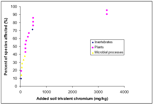
Figure 10. The SSD (plotted as a cumulative frequency against added trivalent chromium (Cr (III)) concentration) of Cr (III) for soil invertebrate species, plant species and soil microbial processes.
Only the Cr (III) toxicity data for E. fetida and E. andrei could be normalised to the Australian reference soil. Thus, a set of generic ACLs and a set of soil-specific ACLs were derived (for the earthworms). The soil-specific ACL values below a clay content of 10% were smaller than the generic ACL values. The soil-specific ACL at a clay content of 10% equalled the generic ACL, and all soil-specific ACLs for soils with a clay content greater than 10% were larger than the generic ACLs. The lower of the soil-specific ACL values and the generic ACL values were adopted as the final ACLs for Cr (III). Thus, the situation was simplified to the soil-specific ACLs only applying up to a clay content of 10% at which point the generic ACL values apply. The generated ACLs for the three land uses and the three types of toxicity data (that is, NOEC and EC10, LOEC and EC30, EC50) are presented in Table 85.
The range between the largest and smallest ACL values generated was approximately 4.0 to 470 mg added Cr (III)/kg. The residential/urban ACLs based on NOEC and EC10, LOEC and EC30, and EC50 data ranged from 3575, 75160, and 110230 mg added Cr (III)/kg respectively.
Table 85. The ACLs based on NOEC and 10% effect concentration (EC10) data, LOEC and 30% effect concentration (EC30), and 50% effect concentration (EC50) toxicity data for trivalent chromium (Cr (III)) for various land uses. These are based on all the Cr (III) toxicity data, except the catalase and nitrogenase enzyme activity data.
Data type | Land use | Clay content | |||
1 | 2.5 | 5 | ≥10 | ||
NOEC | AES | 4 | 6 | 7 | 9 |
| UR | 35 | 45 | 60 | 75 |
| C/I | 65 | 90 | 110 | 140 |
LOEC | AES | 25 | 30 | 40 | 50 |
| UR | 75 | 100 | 130 | 160 |
| C/I | 120 | 170 | 210 | 270 |
EC50 | AES | 9 | 10 | 15 | 20 |
| UR | 110 | 150 | 190 | 230 |
| C/I | 220 | 300 | 375 | 470 |
AES = Areas of ecological significance
UR = urban residential/public open space
C/I = commercial/industrial land uses.
For sites with no history of Cr (III) contamination, the method of Hamon et al. (2004) is recommended to estimate the Cr ABC. Technically this method predicts total Cr but under aerobic soil conditions the vast majority of Cr will be present as Cr (III). It is therefore appropriate to use the Hamon et al (2004) method to estimate Cr (III) ABC values. The equation to predict the Cr ABC is:
log Cr conc (mg/kg) = 0.75 log Fe content (%) + 1.242 (equation 12)
Examples of the ABC values predicted by this equation are presented in Table 86. Predicted ABC values for Cr (III) range from approximately 3 to 160 mg/kg in soils with iron concentrations between 0.1 and 20%.
Table 86. ABCs for chromium (Cr) predicted using the method of Hamon et al. (2004) (equation 12 above).
Fe content (%) | Predicted Cr ABC (mg/kg) |
0.1 | 3 |
0.5 | 10 |
1 | 15 |
2 | 30 |
5 | 60 |
10 | 100 |
15 | 130 |
20 | 160 |
ABC values for Cr (III) vary with soil type (Table 86). Therefore, it is not possible to present a single set of SQG values. Thus, two examples of each of Cr (III) SQG(NOEC & EC10) values, SQG(LOEC & EC30) values and SQG(EC50) values are provided below. These examples would be at the low and high end of the range of SQG values (but not the extreme values) generated for Australian soils.
SQG(NOEC & EC10) Example 1 |
Site descriptors urban residential land/public open space use in a new suburb. Soil descriptors a sandy acidic soil (pH 5, CEC 10, clay content 2.5%) with 1% iron content. The resulting ACL(NOEC & EC10), ABC and SQG(NOEC & EC10) values are: ACL(NOEC & EC10): 45 mg/kg ABC: 15 mg/kg SQG(NOEC & EC10): 60 mg/kg |
SQG(NOEC & EC10) Example 2 |
Site descriptors commercial/industrial land use in a new suburb. Soil descriptors an alkaline clay soil (pH 7.5, CEC 40, clay content 20%) with 10% iron content. The resulting ACL(NOEC & EC10), ABC and SQG(NOEC & EC10) values are: ACL(NOEC & EC10): 140 mg/kg ABC: 100 mg/kg SQG(NOEC & EC10): 240 mg/kg |
SQG(LOEC & EC30) Example 1 |
Site descriptors urban residential land /public open space use in a new suburb. Soil descriptors a sandy acidic soil (pH 5, CEC 10, clay content 2.5%) with 1% iron content. The resulting ACL(LOEC & EC30), ABC and SQG(LOEC & EC30) values are: ACL(LOEC & EC30): 100 mg/kg ABC: 15 mg/kg SQG(LOEC & EC30): 115 mg/kg, which would be rounded off to 110 mg/kg. |
SQG(LOEC & EC30) Example 2 |
Site descriptors commercial/industrial land use/public open space in a new suburb. Soil descriptors an alkaline clay soil (pH 7.5, CEC 40, clay content 20%) with 10% iron content. The resulting ACL(LOEC & EC30), ABC and SQG(LOEC & EC30) values are: ACL(LOEC & EC30): 270 mg/kg ABC: 100 mg/kg SQG(LOEC & EC30): 370 mg/kg |
SQG(EC50) Example 1 |
Site descriptors urban residential land/public open space use in a new suburb. Soil descriptors a sandy acidic soil (pH 5, CEC 10, clay content 2.5%) with 1% iron content. The resulting ACL(EC50), ABC and SQG(EC50) values are: ACL(EC50): 150 mg/kg ABC: 15 mg/kg SQG(EC50): 165 mg/kg, which would be rounded off to 160 mg/kg. |
SQG(EC50) Example 2 |
Site descriptors commercial/industrial land use in a new suburb. Soil descriptors an alkaline clay soil (clay content 20%) with 10% iron content. The resulting ACL(EC50), ABC and SQG(EC50) values are: ACL(EC50): 470 mg/kg ABC: 100 mg/kg SQG(EC50): 570 mg/kg |
There are no ALFs available for Cr (III) nor data available to derive ALFs. Therefore, as an interim measure, the mean of the ALF values available for other cations (that is, Cd, Cu, Co, Ni, Pb and Zn) from Smolders et al. (2009) was determined. This resulted in a value of 2.35[4], which was rounded off to 2.5.
All the Cr (III) toxicity data was multiplied by the ALF of 2.5. Therefore, the aged SQG(NOEC & EC10), SQG(LOEC & EC30) and SQG(EC50) values are exactly 2.5 times the corresponding fresh SQGs for Cr (III). The resulting aged SQG(NOEC & EC10), SQG(LOEC & EC30) and SQG(EC50) values are presented in Table 87.
For aged contaminated sites (that is, the contamination has been in place for at least 2 years, Schedule B5b) the methodology recommends using the 25th percentiles of the ABC data for the ‘old suburbs’ of Olszowy et al. (1995) (see Table 88). Chromium concentrations in old suburbs are higher than those for new suburbs (Olszowy et al. 1995); therefore, it is appropriate to use the ABC values for aged suburbs. The Cr concentrations reported by Olszowy et al (1995) are for total Cr; however, as was the case with the Hamon et al. (2004) method, the majority of the Cr measured will be Cr (III) and thus the data can be used to estimate ABC values for Cr (III). The Olszowy et al. (1995) data was derived from soils low in geogenic Cr and, by using low ABCs, could create low SQGs in some areas with naturally high background Cr concentrations. This problem could be overcome in areas of high natural Cr (III) by using measured ABC values or using the Hamon et al. (2004) method.
Data type | Land use | Clay content | |||
1 | 2.5 | 5 | ≥10 | ||
NOEC | AES | 10 | 15 | 20 | 20 |
| UR | 85 | 120 | 150 | 190 |
| C/I | 170 | 230 | 280 | 360 |
LOEC | AES | 60 | 80 | 100 | 130 |
| UR | 190 | 250 | 310 | 400 |
| C/I | 310 | 420 | 530 | 660 |
EC50 | AES | 25 | 30 | 40 | 50 |
| UR | 275 | 370 | 460 | 580 |
| C/I | 550 | 750 | 940 | 1200 |
AES = Areas of ecological significance, UR = urban residential/public open space, C/I = commercial/industrial land uses.
Table 88. Chromium ABCs based on the 25th percentiles of Cr concentrations in ‘old suburbs’ (that is, >2 years old) from various states of Australia (Olszowy et al. 1995).
Suburb type | 25th percentile of Cr ABC values (mg/kg) | |||
NSW | QLD | SA | VIC | |
Old suburb, low traffic | 8 | 15 | 15 | 10 |
Old suburb, high traffic | 15 | 7 | 15 | 10 |
ABC values for Cr (III) vary with soil type and location (Table 88). Therefore, it is not possible to present a single set of SQG values. Thus, two examples of each of Cr (III) SQG(NOEC & EC10) values, SQG(LOEC & EC30) values and SQG(EC50) values for aged Cr (III) contamination are provided below. These examples would be at the low and high end of the range of SQG values (but not the extreme values) generated for Australian soils.
SQG(NOEC & EC10) Example 1 |
Site descriptors urban residential land /public open space use in an old Victorian suburb with low traffic volume. Soil descriptors a sandy acidic soil (pH 5, CEC 10, clay content 2.5%) with 1% iron content. The resulting ACL(NOEC & EC10), ABC and SQG(NOEC & EC10) values are: ACL(NOEC & EC10): 120 mg/kg ABC: 10 mg/kg SQG(NOEC & EC10): 130 mg/kg |
SQG(NOEC & EC10) Example 2 |
Site descriptors commercial/industrial land use in an old NSW suburb with high traffic volume. Soil descriptors an alkaline clay soil (pH 7.5, CEC 40, clay content 20%) with 10% iron content. The resulting ACL(NOEC & EC10), ABC and SQG(NOEC & EC10) values are: ACL(NOEC & EC10): 360 mg/kg ABC: 15 mg/kg SQG(NOEC & EC10): 375 mg/kg, which would be rounded off to 370 mg/kg. |
SQG(LOEC & EC30) Example 1 |
Site descriptors urban residential land/public open space use in an old Victorian suburb with low traffic volume. Soil descriptors a sandy acidic soil (pH 5, CEC 10, clay content 2.5%) with 1% iron content. The resulting ACL(LOEC & EC30), ABC and SQG(LOEC & EC30) values are: ACL(LOEC & EC30): 250 mg/kg ABC: 10 mg/kg SQG(LOEC & EC30): 260 mg/kg |
SQG(LOEC & EC30) Example 2 |
Site descriptors commercial/industrial land use in an old NSW suburb with high traffic volume. Soil descriptors an alkaline clay soil (pH 7.5, CEC 40, clay content 20%) with 10% iron content. The resulting ACL(LOEC & EC30), ABC and SQG(LOEC & EC30) values are: ACL(LOEC & EC30): 660 mg/kg ABC: 15 mg/kg SQG(LOEC & EC30): 675 mg/kg, which would be rounded off to 670 mg/kg. |
SQG(EC50) Example 1 |
Site descriptors urban residential land/public open space use in an old Victorian suburb with low traffic volume. Soil descriptors a sandy acidic soil (pH 5, CEC 10, clay content 2.5%) with 1% iron content. The resulting ACL(EC50), ABC and SQG(EC50) values are: ACL(EC50): 370 mg/kg ABC: 10 mg/kg SQG(EC50): 380 mg/kg |
SQG(EC50) Example 2 |
Site descriptors commercial/industrial land use in an old NSW suburb with high traffic volume. Soil descriptors an alkaline clay soil (pH 7.5, CEC 40, clay content 20%) with 10% iron content. The resulting ACL(EC50), ABC and SQG(EC50) values are: ACL(EC50): 1200 mg/kg ABC: 15 mg/kg SQG(EC50): 1215 mg/kg, which would be rounded off to 1200 mg/kg. |
The Cr (III) toxicity data set met the minimum data requirements to use the SSD method but there was only one normalisation relationship available (for the earthworm Eisenia fetida) to account for soil characteristics. Based on the criteria for assessing the reliability of SQGs in Schedule B5b, this means that the Cr (III) SQGs were considered to be of moderate reliability.
A compilation of SQGs for Cr (III), Cr (VI) and total Cr from a number of international jurisdictions is presented in Table 89. These guidelines have a variety of purposes and levels of protection and therefore comparison of the values is problematic. The SQGs for Cr (III) range from 2650 mg/kg (total Cr (III)). The majority of jurisdictions do not have SQGs for Cr (III), more typically they have SQGs for total Cr. Carlon (2007), in his review of the SQGs of members of the EU, did not identify whether the SQGs were for added or total Cr, nonetheless they range from 341000 mg/kg. Hexavalent Cr is typically considered to be more toxic than Cr (III) and this is reflected by it having lower SQGs (Table 89).
The ACLs for fresh Cr (III) contamination that apply to urban residential land/public open space land use based on NOEC and EC10, LOEC and EC30, and EC50 data ranged from 3575, 75160 and 100230 mg added Cr (III)/kg respectively. The SQGs based on NOEC and EC10 data are closest to the existing international SQGs for Cr (III). It should be noted that all of the ACLs for urban residential land/public open space land use (irrespective of what data was used to generate them) are considerably smaller than the superseded interim urban EIL of 400 mg total Cr/kg (NEPC 1999). However, the ACLs are consistent with the available Cr (III) toxicity data where there are 6 species/microbial processes that have EC50 values below the superseded interim urban EIL and there are 12 and 16 species/microbial processes that have LOEC and EC30 or NOEC and EC10 data respectively, below the superseded interim urban EIL. The species/microbial processes with toxicity values below the superseded interim urban EIL can be indentified by referring to Table 83.
The ACLs for aged Cr (III) contamination that apply to urban residential land/public open space land use based on NOEC and EC10, LOEC and EC30, and EC50 data ranged from 85190, 175400 and 270580 mg added Cr (III)/kg respectively. None of the ACLs based on NOEC & EC10 and LOEC & EC30 toxicity data were larger than the current interim EIL. However, once the clay content was 5% or above, the ACL values based on EC50 data were larger than the superseded interim EIL. All of the ACLs for aged Cr (III) contamination are considerably larger than the collated international Cr (III) SQGs.
Table 89. Soil quality guidelines (mg/kg) for total chromium, trivalent chromium (Cr (III)) and hexavalent chromium (Cr (VI)) from international jurisdictions.
Name of chromium soil quality guideline | Total chromium | Trivalent chromium | Hexavalent chromium |
Canadian SQG (residential)1 |
|
| 0.4 (total) |
Canadian SQG (commercial and industrial)1 |
|
| 1.4 (total) |
Danish soil quality guideline2 |
| 50 (total) | 2 (total) |
Dutch target value3 | 100 (added Cr) |
|
|
Dutch maximum permissible addition3 | 380 (added Cr) |
|
|
Eco-SSL plants4 |
| ID | ID |
Eco-SSL soil invertebrates4 |
| ID | ID |
Eco-SSL avian4 |
| 26 (total) | ID |
Eco-SSL mammalian4 |
| 34 (total) | 130 (total) |
EU minimal risk values (residential)5 | 34130 (added & total) |
| 2.5 (added & total) |
EU warning risk values (residential)5 | 50450 (added & total) |
| 4.220 (added & total) |
EU potential risk values (residential)5 | 1001000 (added & total) |
|
|
1 = CCME 1999h and 2006 and http://ceqg-rcqe.ccme.ca/
2 = Scott-Fordsmand and Pedersen 1995
3 = VROM 2000
4 = http://www.epa.gov/ecotox/ecossl/
5 = Carlon 2007
ID = insufficient data.
The methodology for deriving SQGs, detailed in Schedule B5b, was implemented to calculate SQGs based on different types of toxicity data for eight contaminants (arsenic, chromium, copper, DDT, lead, naphthalene, nickel, zinc). These eight chemicals were selected as they have a variety of physicochemical properties and, as a result, would behave differently in the environment. They are frequently found in urban Australian contaminated sites. The results of this process are summarised below for each contaminant. Some contaminants have the potential to leach from the contaminated site and thus may cause deleterious effects on groundwater and surface water ecosystems. The fact that contaminants can leach can be taken into account in deriving SQGs. This was done for zinc and arsenic, to illustrate the process and to illustrate the effect that it can have on the resulting SQG.
There was a considerable amount of toxicity data available for the essential element zinc. Zinc does not biomagnify but has the potential to leach from contaminated soil to groundwater. The minimum data requirements to use the SSD method were exceeded, there were multiple normalisation relationships, and there was an ageing/leaching factor. The toxicity data could be expressed in terms of added Zn concentrations; therefore, high reliability soil-specific Zn ACL(NOEC & EC10), ACL(LOEC & EC30) and ACL(EC50) values and corresponding SQG values could be derived for:
Soil-specific ACLs could be derived, so a suite of values were generated. For example, the ACL(NOEC & EC10) values for urban residential/public open space sites freshly contaminated with Zn ranged from 20 (at a cation exchange capacity of 5 and a soil pH of 4) to 330 mg/kg (at a cation exchange capacity of 60 and a soil pH of 7.5). The range of ACL values reflects the ability of different soils to modify the bioavailability and toxicity of Zn. Correcting for ageing led to a marked increase in the ACL values. The corresponding ACL(NOEC & EC10) values for aged Zn contamination range from 45800 mg/kg. As such, correcting for the ageing of Zn led to a more than doubling of the recommended ACL values. The ACL(LOEC & EC30) and ACL(EC50) values were approximately 1.252 and 1.52 times larger, respectively, than the corresponding ACL(NOEC & EC10) values. The lowest of the Zn ACLs for urban residential land/public open space (20 mg/kg) are essentially identical to the lowest corresponding international SQGs, while the higher Zn ACLs are considerably larger than any international SQG.
Arsenic does not biomagnify in oxidised soils but has the potential to leach from contaminated soil to groundwater. Therefore, only the direct toxicity route of exposure needs to be considered in deriving the SQGs. The minimum data requirements to use the SSD method were exceeded, there were no normalisation relationships, and an ageing/leaching factor was available.
The toxicity data could only be expressed in terms of total As concentrations, therefore moderate reliability generic (not soil-specific) As SQG(NOEC & EC10), SQG(LOEC & EC30) and SQG(EC50) values could be derived for:
The generic As SQG(NOEC & EC10) value for soils with areas of ecological significance, urban residential/public open space and commercial/industrial land uses were 8, 20 and 30 mg/kg (total As) respectively. The SQG(LOEC & EC30) and SQG(EC50) values were approximately 2.55 and 3.755 times larger, respectively, than the corresponding SQG(NOEC & EC10) values. The As SQG(NOEC & EC10) for urban residential/public open space soils is identical to the superseded interim urban EIL of 20 mg/kg (NEPC1999). Both the As SQG(NOEC & EC10) and the superseded EIL lie in the lower portion of the range of international As SQGs. The SQG(NOEC & EC10) for aged contamination, at 40 mg/kg, was twice the superseded interim urban EIL for As. The aged As SQG(LOEC & EC30) for urban residential/public open space soils lies in the upper part of the range of international SQGs while the aged As SQG(EC50) value for urban residential/public open space soils is markedly larger than any other international SQG.
Naphthalene does not biomagnify and has only a moderate potential to leach to groundwater. Therefore, only the direct toxicity exposure route was considered in deriving the SQGs. The minimum data requirements to use the SSD method were exceeded, there were no normalisation relationships, and there was no ageing/leaching factor. The toxicity data could only be expressed as total naphthalene concentrations. Therefore, moderate reliability generic (not soil-specific) naphthalene SQG(NOEC & EC10), SQG(LOEC & EC30) and SQG(EC50) values could be derived for:
The generic naphthalene SQG(NOEC & EC10) values for soils with areas of ecological significance, urban residential/public open space and commercial/industrial land uses were 5, 70 and 150 mg/kg (total naphthalene) respectively. The SQG(LOEC & EC30) and SQG(EC50) values were approximately 22.5 and 5 times larger, respectively, than the corresponding SQG(NOEC & EC10) values. There is only a very limited number of international SQGs for naphthalene, which differ markedly (that is, from 0.6 to 125). The SQG(NOEC & EC10) for urban residential/public open space soils of 70 mg/kg is very similar to the top of the EU range of SQGs and in the middle of the range of collated international SQGs.
DDT biomagnifies and has a very low potential to leach to groundwater. Therefore, only the biomagnification and direct toxicity exposure pathways were assessed in deriving SQGs. The minimum data requirements to use the SSD method were exceeded, there were no normalisation relationships, and there was no ageing/leaching factor. The toxicity data could only be expressed as total DDT concentrations. Therefore, moderate reliability generic (not soil-specific) DDT SQG(NOEC & EC10), SQG(LOEC & EC30) and SQG(EC50) could be derived for:
The generic DDT SQG(NOEC & EC10) values for soils with areas of ecological significance, urban residential/public open space and commercial/industrial land uses were 1, 70 and 250 mg/kg (total DDT) respectively. The SQG(LOEC & EC30) and SQG(EC50) values were approximately 2.6 2 and 56 times larger, respectively, than the corresponding SQG(NOEC & EC10) values. The international SQGs for DDT range from 0.01 to 4 mg/kg. The SQG(NOEC & EC10) value for freshly contaminated urban residential/public open space soil is thus considerably larger than the international guidelines but is considerably smaller than the HILs, which range from 260 to 4000 mg/kg (see Schedule B1).
Copper is an essential element. It has a low potential to leach to groundwater. Copper does not biomagnify and therefore only direct toxic effects were considered. There was an extensive toxicity data set for Cu (39 species or soil microbial processes). There were normalisation relationships available for plants, invertebrates and soil microbial processes. An ageing/leaching factor was also available. Therefore high reliability soil-specific ACLs could be derived using NOEC and EC10, LOEC and EC30, and EC50 data for:
The ACL(NOEC and EC10) values for urban residential/public open space sites freshly contaminated with Cu ranged from approximately 20 (at a soil pH of 4.5) to 70 mg added Cu/kg (at a soil pH of 8). Correcting for ageing led to a marked increase in the ACL values. The corresponding ACL values for aged Cu contamination range from 30120 mg added Cu/kg. The range of ACL values reflects the ability of different soils to modify the bioavailability and toxicity of Cu. The ACLs based on LOEC and EC30 data and based on EC50 data were approximately 1.52 and 2.53 times larger, respectively, than the corresponding SQGs based on NOEC and EC10 data. All of the Cu ACLs for residential land use lie within the range of international SQGs for Cu (141000 mg/kg). The superseded interim urban EIL for Cu was 100 mg/kg (total Cu). Therefore the superseded interim EIL for Cu falls within the range of values of all of the SQGs for urban residential land/public open space land uses. The SQGs will permit both considerably less and considerably more Cu in urban residential/public open space soils, depending on the properties of the soils.
Lead is not an essential element but it does not biomagnify in terrestrial ecosystems, nor does it have any significant potential to leach to groundwater. There was toxicity data for 19 species and soil microbial processes which included plants, invertebrates and soil microbial processes. There were no useful normalisation relationships. An ageing/leaching factor has been published in the literature. Therefore moderate reliability generic (not soil-specific) Pb SQGs could be derived using NOEC and EC10, LOEC and EC30, and EC50 data for:
The generic Pb ACL for urban residential/public open space land use that was calculated using NOEC and EC10 data was 130 mg added Pb/kg. The equivalent SQG for aged Pb contamination was 530 mg added Pb/kg. The corresponding ACLs calculated using LOEC and EC30 and using EC50 data were approximately 2 and 4 times larger than the NOEC and EC10 derived ACL values. All the Pb ACLs for urban residential/public open space soils fell within the range of SQGs that have been adopted in other international jurisdictions (25700 mg/kg).
The superseded interim urban EIL was 600 mg/kg (total Pb). All of the Pb SQGs for fresh contamination are lower than the superseded interim urban EIL. The aged SQGs based on NOEC and EC10 are slightly smaller than the superseded interim urban EIL, while the SQGs based on LOEC and EC30 and based on EC50 data are considerably higher.
Nickel does not biomagnify so only the direct toxicity exposure route was considered in deriving the SQGs. Nickel, however, does have the potential to leach to groundwater. There was toxicity data for a total of 53 plant and animal species or soil microbial processes. In addition, there were normalisation relationships available for invertebrates, plants and soil microbial processes. A soil pH-modified ageing/leaching factor was available. The minimum data requirements to use the SSD method were exceeded, there were no normalisation relationships, and there was no ageing/leaching factor. Therefore high reliability soil-specific ACLs could be derived using NOEC and EC10, LOEC and EC30, and EC50 data for:
The soil-specific Ni ACLs based on NOEC and EC10 data for urban residential/public open space soils ranged from 10170 mg added Ni/kg for soils with a CEC ranging from 5 to 60 cmolc/kg. The corresponding ACL values for aged Ni contamination ranged from 15290 mg added Ni/kg. The ACL values based on LOEC and EC30 data and based on EC50 data were essentially identical and approximately 3 times larger than the NOEC and EC10-based ACL values. The range of international SQGs for Ni is 24500 mg/kg. Thus, only the urban residential/public open space ACLs for soils with a CEC above 40 cmolc/kg lie outside the range of internationally adopted SQGs. The superseded interim urban EIL for Ni was 60 mg/kg (total Ni). All of the SQGs would permit both lower and higher concentrations than the superseded interim urban EIL. In soils with a low Ni bioavailability, the maximum recommended concentration of Ni that can be added is 15 times the superseded interim urban EIL.
Trivalent chromium is an essential element for humans and animals but not for plants. It does not pose a potential environmental problem due to leaching (unless it is oxidised to hexavalent chromium), nor does it biomagnify. Toxicity data was available for a total of 21 invertebrate and plant species and soil microbial processes. There were only normalisation relationships available for earthworms. There was no ageing/leaching factor available for Cr (III). Therefore moderate reliability soil-specific ACLs could be derived using NOEC and EC10, LOEC and EC30, and EC50 data for:
The soil-specific Cr (III) ACL values based on NOEC and EC10 data for urban residential/ public open space land uses ranged from 3575 mg added Cr (III)/kg for soils with a clay content from 1 to greater than 10%. The ACL values based on LOEC and EC30 and based on EC50 data were approximately 2 and 3 times larger than the NOEC-based ACLs. The ACLs for aged Cr (III) contamination were approximately 2.5 times larger than the corresponding ACLs for fresh contamination. The ACLs for Cr (III) based on NOEC and EC10 data are consistent with other internationally adopted Cr (III) SQGs. The ACL values based on LOEC and EC30 and on EC50 data are larger than the current international Cr (III) SQGs.
The superseded interim urban EIL for total Cr was 400 mg/kg. This is considerably higher than any of the SQGs for fresh Cr (III) by a factor of at least 2.6. The aged ACLs are essentially 2.5 times larger than the corresponding fresh ACLs.
Adema, DMM & Henzen, L 2001, De Invloed van 50 Prioritaire Stoffen op de Groei van Lactuca sativa (sla.), TNO-Rapport No.21003, TNO, Delft, Netherlands, cited in the ECOTOX database, US EPA 2007.
Aery, NC & Jagetiya, BL 1997, ‘Relative toxicity of cadmium, lead and zinc on barley’, Communications in Soil Science and Plant Analysis, vol. 28, nos 11&12, pp. 949–960.
Ali, NA, Ater, M, Sunahara, G & Robidoux, PY 2004, ‘Phytotoxicity and bioaccumulation of copper and chromium using barley (Hordeum vulgare L.) in spiked artificial and natural forest soils’, Ecotoxicology and Environmental Safety, vol. 57, no. 3, pp. 363–374.
Al-Khafaji, AA & Tabatabai, MA, 1979, ‘Effects of trace elements on arylsuflatase activity in soils’, Soil Science, vol. 127, no. 3, pp. 129–133.
Ambrose, D, Lawrenson, IJ & Sprake, CHS 1975, ‘Vapor-pressure of naphthalene’, Journal of Chemical Thermodynamics, vol. 7, pp. 11731176.
Anastasia, FB, Kender, WJ 1973, ‘The influence of soil arsenic on the growth of lowbush blueberry’, Journal of Environmental Quality, vol. 2, pp. 335337.
ANZECC & ARMCANZ 2000, National water quality management strategy. Australian and New Zealand guidelines for fresh and marine water quality, Australian and New Zealand Conservation Council and Agriculture, & Resource Management Council of Australia and New Zealand.
ATSDR 2002, Toxicological profile for DDT, DDE, and DDD, Public Health Service, Agency for Toxic Substances and Disease Registry, US Department of Health and Human Services, Washington, DC.
ATSDR 2005, Toxicological profile for naphthalene, 1-methyl-naphthalene, and 2-methylnaphthalene, Public Health Service, Agency for Toxic Substances and Disease Registry, US Department of Health and Human Services, Washington, DC.
Augustsson, AK & Rundgren, S 1998, ‘The enchytraeid Cognettia sphagnetorum in risk assessment: advantages and disadvantages’, Ambio, vol. 27, pp. 62–69.
Babich, H & Stotzky, G 1982, ‘Toxicity of nickel to microorganisms in soil: influence of some physicochemical characteristics’, Environmental Pollution, vol. 29, pp. 303–315.
Barry, G & Bell, M 2006, Sustainable biosolids recycling in South-East Queensland. Final project report to Brisbane Water and SEQROC biosolids management project group.
Bartlett, RJ & James, BR 1988, ‘Mobility and bioavailability of chromium in soils’, in Nriagu, JO, Nieboer, E (eds), Chromium in the natural and human environment, pp. 267304, Wiley, New York, USA.
Beeze, VG 1973, ‘Land reclamation and river pollution problems in the coal valley caused by waste from chromate manufacture’, Journal of Applied Ecology, vol. 10, pp. 513–527.
Bengtsson, G, Gunnarsson, T & Rundgren, S 1986, ‘Effects of metal pollution on the earthworm Dendrobaena rubida (Sav.) in acidified soils’, Water, Air, and Soil Pollution, vol. 28, pp. 361–383.
Best, GR, Nabholz, JV, Ojasti, J & Crossley, DA 1978, ‘Response of microarthropod populations to naphthalene in 3 contrasting habitats’, Pedobiologia, vol. 18, pp. 189201.
Bidleman, TF & Foreman, WT 1987, Vapor-particle partitioning of semi-volatile organic-compounds, Advances in Chemistry series, vol. 216, pp. 2756.
Boawn, LC & Rasmussen, PE 1971, ‘Crop response to excessive zinic fertilization of alkaline soil’, Agronomy Journal, vol. 63, pp. 874883.
Bodar, CWM 2007, Environmental risk limits for zinc, RIVM letter report 11235/2007, RIVM (National Institute for Public Health and the Environment), Bilthoven, Netherlands.
Bollag, JM & Barabasz, W 1979, ‘Effect of heavy metals on the denitrification process in soil‘, Journal of Environmental Quality, vol. 8, pp.196201.
Bonet, A, Poschenrieder, C & Barcelo, J, ‘Chromium III-iron interaction in Fe-deficient and Fe-sufficient bean plants, I, growth and nutrient content’, Journal of Plant Nutrition, vol. 14, no. 4, pp. 403414.
Bongers, M, Rusch, B & van Gestel, CAM 2004, ‘The effect of counterion and percolation on the toxicity of lead for the springtail Folsomia candida in the soil‘, Environmental Toxicology and Chemistry, vol. 23, pp. 195–199.
Boyd, WA & Williams, PL 2003, ‘Availability of metals to the nematode Caenorhabditis elegans: toxicity based on total concentrations in soil and extracted fractions’, Environmental Toxicology and Chemistry, vol. 22, pp. 11001106.
Bremner, JM & Douglas, LA 1971, ‘Inhibition of urease activity in soils’, Soil Biology and Biochemistry, vol. 3, pp. 297–307.
Broos, K, Warne, MStJ, Heemsbergen, DA, Stevens, D, Barnes, MB, Correll, RL & McLaughlin, MJ 2007, ‘Soil factors controlling the toxicity of Cu and Zn to microbial processes in Australian soils’, Environmental Toxicology and Chemistry, vol. 26, no. 4, pp. 583590.
Brun, LA, Le Corff, J & Maillet, J 2003, ‘Effects of elevated soil copper on phenology, growth and reproduction of five ruderal plant species’, Environmental Pollution, vol. 122, pp. 361368.
Butler, C, Nash, D, Hannah, M, Cody, J, Warne, MStJ & McLaughlin, MJ 2007, The National Biosolids Research Program – Victoria, final report – June 2007, Victorian Department of Primary Industries, Victoria, Australia.
Campbell, E, Palmer, MJ, Shao, Q, Wilson, D 2000, ‘BurrliOZ: a computer program for the estimation of the trigger values for the ANZECC and ARMCANZ water quality guidelines’, in ANZECC & ARMCANZ 2000, National water quality management strategy. Australian and New Zealand guidelines for fresh and marine water quality, Australian and New Zealand Conservation Council & Agriculture and Resource Management Council of Australia and New Zealand.
Campbell, E, Norstrom, RJ, Hobson, KA, Muir, DCG, Backus, S & Fisk, AT 2005, ‘Mercury and other trace elements in a pelagic Arctic marine food web (Northwater Plynya Baffin Bay)’, Science of the Total Environment, vol. 351, pp. 247–263.
Carlon, C (ed.) 2007, Derivation methods of soil screening values in Europe. A review and evaluation of national procedures towards harmonization, EUR 22805-EN, European Commission, Joint Research Centre, Ispra.
Castro, TF &Yoshida, T 1971, ‘Degradation of organochlorine insecticides in flooded soils in the Philippines’, Journal of Agriculture and Food Chemistry, vol. 19, pp. 168170.
CCME 1999a, Canadian soil quality guidelines for the protection of environmental and human health: zinc, Canadian Council of Ministers of the Environment, Ontario, available online at http://ceqg-rcqe.ccme.ca/download/en/288.
CCME 1999b, Canadian soil quality guidelines for the protection of environmental and human health: arsenic (inorganic), Canadian Council of Ministers of the Environment, Ontario, available online at http://ceqg-rcqe.ccme.ca/download/en/257.
CCME 1999c, Canadian soil quality guidelines for the protection of environmental and human health: naphthalene, Canadian Council of Ministers of the Environment, Ontario, available online at http://ceqg-rcqe.ccme.ca/download/en/271.
CCME 1999d, Canadian soil quality guidelines for the protection of environmental and human health: DDT (total), Canadian Council of Ministers of the Environment, Ontario, available online at http://www.ccme.ca/publications/can_guidelines.html.
CCME 1999e, Canadian soil quality guidelines for the protection of environmental and human health: copper, Canadian Council of Ministers of the Environment, Ontario, available online at http://ceqg-rcqe.ccme.ca/.
CCME 1999f, Canadian soil quality guidelines for the protection of environmental and human health: lead, Canadian Council of Ministers of the Environment, Ontario, available online at http://ceqg-rcqe.ccme.ca/.
CCME 1999g, Canadian soil quality guidelines for the protection of environmental and human health: nickel, Canadian Council of Ministers of the Environment, Ontario, available online at http://ceqg-rcqe.ccme.ca/.
CCME 1999h, Canadian soil quality guidelines for the protection of environmental and human health: chromium, Canadian Council of Ministers of the Environment, Ontario, available online at http://ceqg-rcqe.ccme.ca/.
CCME 2006, A protocol for the derivation of environmental and human health soil quality guidelines, Canadian Council of Ministers of the Environment, Manitoba, available online at http://www.ccme.ca/assets/pdf/sg_protocol_1332_e.pdf.
Cervantes, C, Campos-Garcia J, Devars, S, Guatierrex-Corrora, F, Loza-Tavera, M & Torres-Guzman, JC 2001, ‘Interactions of chromium with microorganisms and plants’, FEMS Micribiology Reviews, vol. 25, pp. 335347.
Chang, FH & Broadbent, FE 1981, ‘Influence of trace-metals on carbon-dioxide evolution from a Yolo soil‘, Soil Science, vol. 132, pp. 416421.
Chang, FH & Broadbent, FE 1982, ‘Influence of trace metals on some soil nitrogen transformations’, Journal of Environmental Quality, vol. 11, pp.14.
Chapman, PM, McDonald, BG, Kickham, PE & McKinnon, S 2006, ‘Global differences in marine metals toxicity’, Marine Pollution Bulletin, vol. 52, pp. 1081–1084.
Chhabra, RJ, Pleysier, J & Cremers, AC 1975, ‘The measurement of the cation exchange capacity and exchangeable cations in soils: a new method’, Proceedings of International Clay Conference, Mexico City, July 16–23, pp. 439449, Applied Publishing, Wilmette, IL, USA.
Chisholm, D & MacPhee, AW, 1972, ‘Persistene and effects of some pesticides in soil’, Journal of Economic Entomology, vol. 65, pp. 10101115.
Clements, HF & Munson, J 1947, ‘Arsenic toxicity studies in soil and in culture solution’, Pacific Science, vol. 1, pp. 151171.
Cooper, HE, Paden, WR, Hall, EE, Albert, WB, Rogers, WB & Riley, JA 1931, ‘Effect of calcium arsenate on the productivity of certain soil types’, South Carolina Agric. Exp. Sta.Ann., Rep. 44, cited by NRC 1977, pp. 2836.
Criel, P, Lock, K, Van Eeckhout, H, Oorts K, Smolders, E & Janssen, CR 2008, ‘Influence of soil properties on copper toxicity for two soil invertebrates‘, Environmental Toxicology and Chemistry, vol. 27, pp. 1748–1755.
Crommentuijn, T, Sijm, D, de Bruijn, J, van den Hoop, M, van Leeuwen, K & van de Plassche, E 2000, ‘Maximum permissible and negligible concentrations for metals and metalloids in the Netherlands, taking into account background concentrations’, Journal of Environmental Management, vol. 60, pp. 121143.
Cunningham, JD, Keeney, DR & Ryan, JA 1975, ‘Phytotoxicity and uptake of metals added to soils as inorganic salts or in sewage sludge’, Journal of Environmental Quality, vol. 4, pp. 460–462.
Dang, YP, ChhabraR & Verma, KS 1990, ‘Effect of Cd, Ni, Pb and Zn on growth and chemical composition of onion and fenugreek’, Communications in Soil Science and Plant Analysis, vol. 21, nos 9 & 10, pp. 717–735.
Davies, NA, Hodson, ME & Black, S 2003a, ‘Is the OECD acute worm toxicity environmentally relevant? The effect of mineral form on the calculated lead toxicity‘, Environmental Pollution, vol. 121, pp. 4954.
Davies, NA, Hodson, ME & Black, S 2003b, ‘Changes in toxicity and bioavailability of lead in contaminated soils to the earthworm Eisenia fetida after bone meal amendments to the soil‘, Environmental Toxicology and Chemistry, vol. 21, no. 12, pp. 2685–2691.
Davis, RD, Beckett, EHT & Wollan, E 1978, ‘Critical levels of twenty potentially toxic elements in young spring barley‘, Plant and Soil, vol. 49, pp. 395408.
De Haan, SD, Rethfeld, H & van Driel, W 1985, ‘Acceptable levels of heavy metals (Cd, Cr, Cu, Ni, Pb, Zn) in soils, depending on their clay and humus content and cation-exchange capacity’, Rapport, Instituut voor Bodemvruchtbaarheid, vol.9, no. 85.
Demayo, A, Taylor, MC, Taylor, KW & Hodson, PV 1982, ‘Toxic effects of lead and lead compounds on human health, aquatic life, wildlife, plants, and livestock’, CRC Critical Reviews in Environmental Control, vol. 12, pp. 257–305.
Deuel, LE & Swoboda, AR 1972, ‘Arsenic toxicity to cotton and soybeans’, Journal of Environmental Quality, vol. 1, pp. 317320.
Doelman P & Haanstra, L 1979, ‘Effect of lead on soil respiration and dehydrogenase activity‘, Soil Biology and Biochemistry, vol. 11, pp. 475–479.
Doelman P & Haanstra, L 1983, cited in van de Meent et al. 1990.
Doelman P & Haanstra, L 1984, ‘Short-term and long-term effects of cadmium, chromium, copper, nickel, lead and zinc on soil microbial respiration in relation to abiotic soil factors‘, Plant and Soil, vol. 79, pp. 317–327.
Doelman P & Haanstra, L 1986, ‘Short-term and long-term effects of heavy-metals on urease activity in soils’, Biology and Fertility of Soils, vol. 2, pp. 213218.
Doelman P & Haanstra, L 1989, ‘Short-term and long-term effects of heavy metals on phosphatase activity in soils: an ecological dose-response model approach‘, Biology and Fertility of Soils, vol. 8, pp. 235–241.
DPIWE 1999, Tasmanian biosolids reuse guidelines, Department of Primary Industry, Water and Environment, Hobart, Tasmania.
Dreyfuss, J 1964, ‘Characterisation of a sulphate and thiosulfate transporting system in Salmonella typhimurium’, Journal of Biological Chemistry, vol. 239, pp. 22922297.
ECB 2003, Technical guidance document on risk assessment, EUR 20418 EN/1, European Chemicals Bureau, Office for Official Publications of the European Community, Luxembourg.
EC 1996, Technical guidance document in support of commission directive 93/67/EEC on risk assessment for new notified substances and commission regulation (EC) no. 1488/94 on risk assessment for existing substances, part II: environment, European Commission, Office for Official Publications of the European Communities, Luxembourg.
EC 2008a, European Union voluntary risk assessment report: copper, copper II sulphate pentahydrate, copper(I)oxide, copper(II)oxide, dicopper chloride trihydroxide. Chapter 3.2: Environmental effects, European Commission, Brussels, Belgium, available online at http://echa.europa.eu/chem_data/transit_measures/vrar_en.asp.
EC 2008b, European Union voluntary risk assessment report: nickel and nickel compounds. Section 3.2: Effects assessment, 2009, European Commission, Brussels, Belgium.
Eisler, R 1988, Lead hazards to fish, wildlife, and invertebrates: a synoptic review, Biological report no. 85, US Fish and Wildlife Service, Laurel, Maryland, USA.
Fendorf, S, La Force, MJ & Li, GC 2004, ‘Temporal changes in soil partitioning and bioaccessability of arsenic, chromium and lead’, Journal of Environmental Quality, vol. 33, pp. 20492055.
Frossard, R, Stadelmann, FX & Niederhauser, J 1989, ‘Effect of different heavy metals on fructan, sugar and starch content of ryegrass’, Journal of Plant Physiology, vol. 134, pp. 180–185.
Frostegård, Å, Tunlid, A & Bååth, E 1993, ‘Phosholipid fatty acid composition, biomass and activity of microbial communities from two soil types experimentally exposed to different heavy metals’, Applied and Environmental Microbiology, vol. 59, pp. 3605–3617.
Fu, MH & Tabatabai, MA 1989, ‘Nitrate reductase activity in soils: effect of trace metals’, Soil Biology and Biochemistry, vol. 21, no. 7, pp. 943–946.
Furlong, CB 1978, Effects of arsenic in the Canadian environment, Publication no. NRCC15391, National Research Council of Canada, Ottawa.
GDCH 1992, ‘Gesellschaft Deutscher Chemiker, Methynaphthalenes’, in GDCH-Advisory Committee on existing chemicals of environmental relevance (BUA), BUA report 47, cited in ATSDR, 2005.
Gupta, SK, Hani, H, Santschi, E & Stadelmann, FX 1987, ‘The effect of graded doses of nickel on the yield, the nickel content of lettuce and the soil respiration’, Toxicological and Environmental Chemistry, vol. 14, pp. 1–9.
Haanstra, L & Doelman, P 1984, ‘Glutamic acid decomposition as sensitive measure of heavy metal pollutin in soil’, Soil Biology and Biochemistry, vol. 16, no.6, pp. 595–600.
Haanstra, L & Doelman, P 1991, ‘An ecological dose-response model approach to short-term and long-term effects of heavy-metals on arylsulfatase activity in soil‘, Biology and Fertility of Soils, vol. 11, pp. 1823.
Halstead, RL, Finn, BJ & MacLean, AJ 1969, ’Extractability of nickel added to soils and its concentration in plants‘, Canadian Journal of Soil Science, vol. 49, pp. 335–342.
Hamon, RE, McLaughlin, MJ, Gilkes, RJ, Rate, AW, Zarcinas, B, Robertson, A, Cozens, G, Radford, N & Bettenay, L 2004, ‘Geochemical indices allow estimation of heavy metal background concentrations in soils’, Global Biogeochemical Cycles, vol. 18, pp. 16.
Hamon, R, Stevens, D & McLaughlin, M 2003, Determination of rates of long-term reactions decreasing bioavailability of zinc and lead in soils, pp. 49, Final report to the International Lead Zinc Research Organisation.
Han, FX, Sridhar, BBM, Monts, DL & Su, Y 2004, ‘Phytoavailability and toxicity of trivalent and hexavalent chromium to Brassica juncea’, New Phytologist, vol. 162, pp. 489–499.
Hansch, C, Leo, A & Hoekman, D 1995, Exploring QSAR - hydrophobic, electronic, and steric constants, American Chemical Society, Washington, DC, USA.
Heemsbergen, D, Broos, K, Whatmuff, M, Warne, MStJ, McLaughlin, M, Stevens, D, Smart, M, Fiebiger, C, Baldock, C, Cozens, G, Tomczak, B & Daly, A 2007, Final report for the South Australian component of the national biosolids research program, CSIRO Land and Water Science Report, 21/07.
Heemsbergen, D, Warne, M, McLaughlin, M & Kookana, R 2008, The Australian methodology to derive ecological investigation levels in contaminated soils 2009, CSIRO Land and Water Science Report 15/08, CSIRO Land and Water, Urrbrae, Australia. (Available online at http://www.clw.csiro.au/publications/science/2008/sr18-08.pdf). Adopted as Schedule B5b in National Environment Protection (Assessment of Site Contamination) Measure 2011, as varied.
Heemsbergen, D, Warne, MStJ, McLaughlin, MJ & Kookana, R 2009, Soil quality guidelines for arsenic, DDT, naphthalene and zinc, CLW Science Report no. 02/09, prepared for the NSW DECCW Environmental Trust.
Hemida, SK, Omar, SA & Abdel Malek, AY 1997, ‘Microbial populations and enzyme activity in soil treated with heavy metals’, Water Air and Soil Pollution, vol. 95, pp. 1322.
Henny, CJ, Blus, LJ, Hoffman, DJ, Grove, RA & Hatfield, JS 1991, ‘Lead accumulation and osprey production near a mining site on the Coeur d’Alene River, Idaho’, Archives of Environmental Contamination and Toxicology, vol. 21, pp. 415–424.
Herbert, IN, Svendsen, C, Hankard, PK & Spurgeon, DJ 2004, ‘Comparison of instantaneous rate of population increase and critical-effect estimates in Folsomia candida exposed to four toxicants’, Ecotoxicology and Environmental Safety, vol. 57, pp. 175–183.
Hiltbold, AE 1975, ‘Behaviour of organoarsenicals in plants and soils’, in Woolson, EA (ed.), Arsenical pesticides, Amer Chem Soc Symp Ser 7, American Chemical Society, Washington, DC, cited by Furlong, 1978, pp. 124147.
Howard, P & Meylan, W (eds) 1997, Handbook of physical properties or organic chemicals, CRC Press, Boca Raton, Florida, USA.
Hooftman, RN & Henzen, L 1996, cited in Bodar, CWM 2007, Environmental risk limits for zinc, RIVM letter report 11235/2007, RIVM (National Institute for Public Health and the Environment), Bilthoven, Netherlands.
HSDB 2004, Hazardous substances data bank, available online at http://toxnet.nlm.nih.gov/cgi-bin/sis/htmlgen?HSDB.htm.
Hund-Rinke, K & Simon, M 2005, ‘Terrestrial ecotoxicity of eight chemicals in a systematic approach’, Journal of Soils and Sediments, vol. 5, pp. 5965.
Jacobs, LW & Keeney, DR 1970, ‘Arsenic phosphorus interactions on corn-M’, Communications in Soil Science and Plant Analysis, vol. 1, pp. 8593.
Jacobs, LW, Keeney, DR & Walsh, LM 1970, ‘Arsenic residue toxicity to vegetable crops grown on plainfield sand’, Agronomy Journal, vol. 62, pp. 588.
Jarvis, SC 1978, ‘Copper uptake and accumulation by perennial ryegrass growth in soil and solution culture’, Journal of Science Food Agriculture, vol. 29, pp.12–18.
Jonker, MJ, Sweijen, R & Kammenga, JE 2004, ‘Toxicity of simple mixtures to the nematode Caenorhabditis elegans in relation to soil sorption’, Environmental Toxicology and Chemistry, vol. 23, pp. 480488.
Juma, NG, Tabatabai, MA 1977, ‘Effects of trace metals on phosphatise activity in soils‘, Soil Science Society of America Journal, vol. 41, pp. 343346.
Kalyanaraman, SB & Sivagurunathan, P 1993, ‘Effect of cadmium, copper, and zinc on the growth of Blackgram’, Journal of Plant Nutrition, vol. 16, pp. 20292042.
Kammenga, JE, Van Koert, PHG, Riksen, JAG, Korthals, GW & Bakker, J 1996, ‘A toxicity test in artificial soil based on the life-history strategy of the nematode Plectus acuminatus‘, Environmental Toxicology and Chemistry, vol. 15, pp. 722–727.
Kegley, SE, Hill, BR, Orme, S & Choi, AH 2008, PAN Pesticide database, Pesticide Action Network, North America, available online at: http://www.pesticideinfo.org.
Keller, E 1970, ‘The DDT story’, Chemistry, vol. 43, pp. 812.
Kenaga, EE 1980, ‘Predicted bioconcentration factors and soil sorption coefficients of pesticides and other chemicals’, Ecotoxicology and Environmental Safety, vol. 4, pp. 2638.
Khan, DH & Frankland, B 1983, ‘Effects of cadmium and lead on radish plants with particular reference to movement of metals through soil profile and plant’, Plant and Soil, vol. 70, pp. 335–345.
Khan, DH & Frankland, B 1984, ‘Cellulolytic activity and root biomass production in some metal-contaminated soils’, Environmental Pollution, Series A, vol. 33, pp.63–74.
Khan, M & Scullion, J 2002, ‘Effects of metal (Cd, Cu, Ni, Pb or Zn) enrichment of sewage-sludge on soil microorganisms and their activities’, Applied Soil Ecology, vol. 20, pp. 145–155.
Kjær, C & Elmegaard, N 1996, ‘Effects of copper sulfate on Black Bindweed (Polygonum convolvulus L.)’, Ecotoxicology and Environmental Safety, vol. 33, pp. 110–117.
Korthals, GW, van de Ende, A, van Megen, H, Lexmond, TM, Kammenga, JE & Bongers, T 1996, ‘Short-term effects of cadmium, copper, nickel and zinc on soil nematodes from different feeding and life-history strategy groups’, Applied Soil Ecology, vol. 4, pp. 107117.
Krogh, PH & Axelsen, JA 1998, ‘Test on the predatory mite Hypoaspis aculeifer preying on the collembolan Folsomia fimetaria’, in Lokke, H & van Gestel, CAM (eds), Handbook of soil invertebrate toxicity tests, pp. 239251, John Wiley and Sons Ltd, Chichester, UK.
Kula, H & Larink, O 1997, ‘Development and standardization of test methods for the prediction of sublethal effects of chemicals on earthworms’, Soil Biology and Biochemistry, vol. 29, pp. 635–639.
Kwok, KWH, Leung, KMY, Chu, VKH, Lam, PKS, Morritt, D & Maltby, L. 2007, ‘Comparison of tropical and temperate freshwater species sensitivities to chemicals: implications for deriving safe extrapolation factors’, Integrated Environmental Assessment and Management, vol. 3, no. 1, pp. 4967.
Langdon, CJ, Piearce, TG, Meharg, AA & Semple, KT 2001, ‘Survival and behaviour of the earthworms Lumbricus rubellus and Dendrodrilus rubidus from arsenate-contaminated and non-contaminated sites’, Soil Biology & Biochemistry, vol. 33, pp. 12391244.
Langdon, CJ, Piearce, TG, Meharg, AA & Semple, KT 2003, ‘Interactions between earthworms and arsenic in the soil environment: a review’, Environmental Pollution, vol. 124, pp. 361373.
Langdon, K, Warne, MStJ & Sunderam, RIM 2009, ‘A compilation of data on the toxicity of chemicals to species in Australasia. Part 4: Metals (20022009)’, Australasian Journal of Ecotoxicology, vol. 15, pp. 51184.
Lapointe, D & Couture, P 2006, Importance of the route of exposure in accumulation and subcellular partitioning of nickel in fathead minnows (Pimephales promelas), Presentation P484 at the 27th Annual Meeting of the Society for Environmental Toxicology and Chemistry Montreal, Quebec, November.
LDA 2008, European union voluntary risk assessment report: lead metal, lead oxide, lead tetroxide and lead stabiliser compounds, Lead Development Association, available online at http://echa.europa.eu/chem_data/transit_measures/vrar_en.asp.
Lexmond, TM, Edelman, T & van Driel, W 1986, ‘Voorlopige referentiewaarden en huidige achtergrondgehalten voor een antal zware metalen en arseen in de bovengrond van natuurterreinen en landbouwgronden’ in Advies Bodemkwaliteit, VTCB A86/02, Ministerie van Volkshuisvesting, Ruimtelijke Ordening en Milieubeheer, Leidschendam, Netherlands.
Liang, CN & Tabatabai, MA 1977, ‘Effects of trace elements on nitrogen mineralisation in soils’, Environmental Pollution, vol. 12, pp. 141147.
Liang, CN & Tabatabai, MA 1978, ‘Effects of trace elements on nitrification in soils’, Journal of Environmental Quality, vol. 7, pp. 291293.
Liang, J & Schoenau, JJ 1995, ‘Development in resin membranes as a sensitive indicator of heavy metal toxicity in the soil environment’, International Journal of Environmental Analytical Chemistry, vol. 59, pp. 265–275.
Lichenstein, E & Schulz, K 1959, ‘Persistence of some chlorinated hydrocarbon insecticides as influenced by soil types, rate of application and temperature’, Journal of Economic Entomology, vol. 52, pp. 124131.
Lighthart, B, Baham, J & Volk, VV 1983, ‘Microbial respiration and chemical speciation in metal-amended soils’, Journal of Environmental Quality, vol. 12, pp. 543548.
Lock, K & Janssen, CR 2001, ‘Modelling zinc toxicity for terrestrial invertebrates’, Environmental Toxicology and Chemistry, vol. 9, pp. 19011908.
Lock, K & Janssen, CR 2002, ‘Ecotoxicity of nickel to Eisenia fetida, Enchytraeus albidus and Folsomia candida’, Chemosphere, vol. 46, pp. 197–200.
Louma, S & Rainbow, PS 2008, Metal contamination in aquatic environments: science and lateral management, Cambridge University Press, England.
Lu, P-Y, Metcalf, R, Furman, R, Vogel, R & Hassett, J 1975, ‘Model ecosystem studies of lead and cadmium and of urban sewage sludge containing these elements’, Journal of Environmental Quality, vol. 4, pp. 505–509.
Luo, YM & Rimmer, DL 1995, ‘Zinc copper interaction affecting plant-growth on a metal-contaminated soil’, Journal of Environmental Pollution, vol. 88, pp. 7983.
Ma, WC 1982, ‘The influence of soil properties and worm-related factors on the concentration of heavy metals in earthworms’, Pedobiologia, vol. 24, pp.109–119.
Ma, WC 1984, ‘Sublethal toxic effects of copper on growth, reproduction and litter breakdown activity in the earthworm Lumbricus rubellus, with observations on the influence of temperature and soil pH’, Environmental Pollution, Series A, Ecological and biological, vol. 33, pp. 207–219.
Maclean, AJ 1974, ‘Effects of soil properties and amendments on availability of zinc in soils’, Canadian Journal of Soil Science, vol. 54, pp. 369378.
MacPhee, AW, Chisholm, D & MacEachern, CR 1960, ‘The persistence of certain pesticides in the soil and their effect on crop yields’, Canadian Journal of Soil Science, vol. 40, pp. 5962.
Markich, SJ, Warne, MStJ, Westbury, A-M & Roberts, CJ 2002, ‘A compilation of data on the toxicity of chemicals to species in Australasia. Part 3: Metals’, Australasian Journal of Ecotoxicology, vol. 8, no. 1, pp. 1–138.
McGrath 1982, cited in Scott-Fordsmand JJ & Pedersen, MB 1995.
McGrath, SP & Smith, S 1990, ‘Chromium and nickel’, in Alloway, BJ (ed.), pp. 125150, Heavy metals in soils, Wiley, New York, USA.
Meharg, AA, Shore, RF & Broadgate, K 1998, ‘Edaphic factors affecting the toxicity and accumulation of arsenate in the earthworm Lumbricus terrestris’, Environmental Toxicology and Chemistry, vol. 17, pp. 11241131.
Metwally, AI & Rabie, MH 1989, ‘Effect of Ni addition on plant growth and nutrient uptake in two soils’, Egyptian Journal of Soil Science, vol. 29, no. 3, pp. 261–274.
Millhollon, RW 1970, ‘MSMA for Johnson grass control in sugarcane‘, Weed Science, vol. 18, pp. 333336.
Molnar, L, Fischer, E & Kallay, M 1989, ‘Laboratory studies on effect, uptake and distribution of chromium in Eisenia fetida (annelida, oligochaeta), Zoologischer Anzeiger, vol. 223, no.1/2, pp. 57–66.
Mortveldt, JJ & Giordano, PM 1975, ‘Response of corn to zinc and chromium in municipal wastes applied to soil’, Journal of Environmental Quality, vol. 4, pp. 170–174.
Muir, D, Wang, X, Bright, D, Lockhart, L & Kock, G 2005, ‘Spatial and temporal trends on mercury and other metals in landlocked char from lakes in the Canadian Arctic archipelago’, Science of the Total Environment, pp. 351352, 464–478.
Nan, Z, Zhao, C, Li, J, Chen, F & Sun, W 2002, ‘Relations between soil properties and selected heavy metal concentrations in spring wheat (Triticum aesitivum L.) grown in contaminated soils‘, Water, Air and Soil Pollution, vol. 133, pp. 205213.
NRC 1977, Arsenic, Printing and Publishing Office, National Research Council, National Academy of Sciences, Washington, DC, USA.
Necker, U & Kunze, C 1986, ‘Incubation experiments on nitrogen mineralisation by fungi and bacteria in metal-amended soil’, Anegwandte Botanik, vol. 60, pp. 8194.
NEPC 1999, ‘Schedule B(1) Guideline on the investigation levels for soil and groundwater’, National Environment Protection (Assessment of Site Contamination) Measure 1999, National Environment Protection Council, Adelaide, Australia.
Olszowy, H, Torr, H & Imray, P 1995, Trace element concentrations in soils from rural and urban areas of Australia, Contaminated sites monograph series no. 4, South Australian Health Commission, Adelaide, Australia.
OMEE 1993, Candidate substances for bans, phase-outs or reductions: Report, Multimedia revision, Ontario Ministry of Environment and Energy, Toronto, Canada.
Oorts, K, Ghesquiere, U, Swinnen, K & Smolders, E 2006a, ‘Soil properties affecting the toxicity of CuCl2 and NiCl2 for soil microbial processes in freshly spiked soils’, Environmental Toxicology and Chemistry, vol. 25, pp. 836844.
Oorts, K, Bronckaer, S & Smolders, E 2006b, ‘Discrepancy of the microbial response to elevated copper between freshly spiked and long-term contaminated soils’, Environmental Toxicology and Chemistry, vol. 25, no. 3, pp. 845–853.
O'Neil, MJ (ed.) 2001, The Merck index - an encyclopedia of chemicals, drugs, and biologicals, 13th edn, Merck and Co, Whitehouse Station, NJ, USA.
Outridge, PM & Scheuhammer, AM 1993, ‘Bioaccumulation and toxicology of nickel: Implications for wild animals and birds’, Environmental Reviews, vol. 1, no. 2, pp. 172–197.
Parks, JL, McNeil, L, Frey, M & Eaton, AD 2004, ‘Determination of total chromium in environmental water samples’, Water Research, vol. 38, pp. 2827–2838.
Patterson, JBE 1971, Trace elements in soils and crops, MAFF Technical Bulletin no. 21, cited in Scott-Fordsmand, JJ & Pedersen, MB 1995, Soil quality criteria for selected inorganic compounds, Report no. 48, Danish Environment Protection Agency, Ministry of Environment and Energy, Denmark.
Pearlman, RS, Yalkowsky, SH, Bannerjee, S 1984, ‘Water solubilities of polynuclear aromatic and heteroaromatic-compounds’, Journal of Physical and Chemical Reference Data, vol. 13, pp. 555562.
Pedersen, MB, van Gestel, CAM & Elmegaard, N 2000a, ‘Effects of copper on reproduction of two Collembolan species exposed through soil, food and water‘, Environmental Toxicology and Chemistry, vol. 19, no. 10, pp. 2579–2588.
Pedersen, MB, Kjaer, C, Elmegaard, N 2000b, ‘Toxicity and bioaccumulation of copper to Black Bindweed (Fallopia convolvulus) in relation to bioavailability and the age of soil contamination’, Archives of Environmental Contamination and Toxicology, vol. 39, pp. 431–439.
Pedersen, MB & van Gestel, CAM 2001, ‘Toxicity of copper to the Collembolan Folsomia fimetaria in relation to the age of soil contamination’, Ecotoxicology and Environmental Safety, vol. 49, pp. 54–59.
Premi, PR & Cornfield, AH 1969, ‘Effects of addition of copper, manganese, zinc and chromium compounds on ammonification and nitrification during incubation of soil‘, Plant and Soil, vol. 31, pp. 345352.
Quraishi, MSI & Cornfield, AH 1973, ‘Incubation study of nitrogen mineralisation and nitrification in relation to soil pH and level of copper (II) addition’, Environmental Pollution, pp. 159–163.
Raab, HE 1972a, Weed Science Society of America - Abstract. pp. 32, cited in Sheppard (1992).
Raab, HE 1972b, Weed Science Society of America - Abstract. pp. 32, cited in Sheppard (1992).
Ray, B 1975, International Pest Control, vol. 17, no. 9, cited in Sheppard (1992).
Rayment, GE & Higginson, FR 1992, ‘Ion-exchange properties’ in Australian laboratory handbook of soil and water chemical methods, pp. 137-194, Inkata, Melbourne, Australia.
Rhoads, FM, Olson, SM & Manning, A 1989, ‘Copper toxicity in tomato plants’, Journal of Environmental Quality, vol. 18, pp. 195–197.
Rooney, C, Zhao, FJ & McGrath, SP 2006, ‘Soil factors controlling the expression of copper toxicity to plants in a wide range of European soils’, Environmental Toxicology and Chemistry, vol. 25, pp. 726–732.
Rooney, C, Zhao, F–J & McGrath, SP 2007, ‘Phytotoxicity of nickel in a range of European soils: Influence of soil properties, Ni solubility and speciation’, Journal of Environmental Pollution, pp. 145, pp. 596–605.
Rosenfels, RS & Crafts, AS 1940, ‘Toxicity studies with arsenic in eighty California soils’, Hilgardia, vol. 12, pp. 177200.
Ross, DS, Sjrogren, RE & Bartlett, RJ 1981, ’Behaviour of chromium in soils. IV. Toxicity to microorganisms’, Journal of Environmental Quality, vol. 10, no. 2, pp. 145–148.
Rothamsted 2005, NiPERA research project on the ‘Development of a predictive model of bioavailability and toxicity of Nickel in soils: Plant toxicity’, cited in EC (2008b), European Union voluntary risk assessment report: nickel and nickel compounds. Section 3.2: Effects assessment, 2009, European Commission, Brussels, Belgium.
Rundgren, S & van Gestel, CAM 1998, ‘Comparison of species sensitivity’, in Lokke, H, van Gestel, CAM (eds), Handbook of soil invertebrate toxicity tests, J Wiley and Sons Ltd, Chichester, UK.
Samborska, A, Stepniewska, Z & Stepniewski, W 2004, ‘Influence of different oxidation states of chromium (VI, III) on soil urease activity’, Geoderma, vol. 122, pp. 317–322.
Sandberg, GR & Allen, IK 1975, ‘An arsenic cycle in an agronomic ecosystem’, in Woolson, EA (ed.), Arsenical pesticides, American Chemical Society Symposium Series 7, American Chemical Society, Washington, DC, cited in Furlong, CB 1978, Effects of arsenic in the Canadian environment, Publication no. NRCC15391, National Research Council of Canada, Ottawa, pp. 124147.
Sandifer, RD & Hopkin, SP 1996, ‘Effects of pH on the toxicity of cadmium, copper, lead and zinc to Folsomia candida Willem, 1902 (Collembola) in a standard laboratory test system‘, Chemosphere, vol. 33, pp. 24752486.
Sandifer, RD & Hopkin, SP 1997, ‘Effects of temperature on the relative toxicities of Cd, Cu, Pb, and Zn to Folsomia candida (Collembola)’, Ecotoxicology and Environmental Safety, vol. 37, pp. 125130.
Saviozzi, A, LeviMinzi, R, Cardelli, R & Riffaldi, R 1997, ‘The influence of heavy metals on carbon dioxide evolution from a typic xerochrept soil‘, Water Air and Soil Pollution, vol. 93, pp. 409417.
Scoccianti, V, Crinelli, R, Tirilline, B, Mancinelli, V & Speranza, A 2006, ‘Uptake and toxicity of Cr (III) in celery seedlings’, Chemosphere, vol. 64, pp.1695–1703.
Scott-Fordsmand, JJ, Krogh, PH & Weeks, JM 1997, ‘Sublethal toxicity of copper to a soil-dwelling springtail (Folsomia fimetaria) (Collembola: Isotomidae)’, Environmental Toxicology and Chemistry, vol. 16, pp. 2538–2542.
Scott-Fordsmand, JJ & Pedersen, MB 1995, Soil quality criteria for selected inorganic compounds, Report no. 48, Danish Environment Protection Agency, Ministry of Environment and Energy, Denmark.
Scott-Fordsmand, JJ, Weeks, JM & Hopkin, SP 1998, ‘Toxicity of nickel to the earthworm and the applicability of the neutral red retention assay’, Ecotoxicology, vol. 7, pp. 291–295.
Scott-Fordsmand, JJ, Weeks, JM & Hopkin, SP 2000, ‘Importance of contamination history for understanding toxicity of copper to earthworm Eisenia fetida (Oligochaeta: Annelida), using neutral red retention assay‘, Environmental Toxicology and Chemistry, vol. 19, no. 7, pp. 1774–1780.
Seiler, JR, Paganelli, DJ 1987, ‘Photosynthesis and growth-response of red spruce and loblolly-pine to soil-applied lead and simulated acid-rain‘, Forest Science, vol. 33, no. 3, pp. 668–675.
Sheppard, MI, Sheppard, SC & Thibault, DH 1982, Identification of the problem phytotoxicant in soil from a radioactive waste disposal area, Report WNRE-461, Atomic Energy of Canada Limited, Pinawa, Manitoba.
Sheppard, MI, Thibault, DH & Sheppard, SC 1985, ‘Concentrations and concentration ratios of U, As, and Co in Scots pine grown in a waste soil and an experimentally contaminated soil’, Water, Air and Soil Pollution, vol. 26, no. 1, pp. 8594.
Sheppard, SC 1992, ‘Summary of phytotoxic levels of soil arsenic’, Water Air and Soil Pollution, vol. 64, pp. 539550.
Shiu, WY & Mackay, D 1997, ‘Henry's law constants of selected aromatic hydrocarbons, alcohols, and ketones’, Journal of Chemical and Engineering Data, vol. 42, pp. 2730.
Sivakumar S & Subbhuraam, CV 2005, ‘Toxicity of chromium (III) and chromium (VI) to the earthworm Eisenia fetida’, Ecotoxicology and Environmental Safety, vol. 62, pp. 93–98.
Skujinš, J, Nohrstedt, H-O, Odén, S 1986, ‘Development of a sensitive biological method for the determination of a low-level toxic contamination in soils‘, Swedish Journal of Agriculture, vol. 16, pp. 113–118.
Smit, CE, Schouten, AJ, Vvn den Brink, PJ, van Esbroek, MLP & Posthuma, L 2002, ‘Effects of zinc contamination on a natural nematode community in outdoor soil mesocosms‘, Archives of Environmental Contamination and Toxicology, vol. 42, pp. 205216.
Smit, CE & van Gestel, CAM 1998, ‘Effects of soil type, prepercolation, and ageing on bioaccumulation and toxicity of zinc for the springtail Folsomia candida‘, Environmental Toxicology and Chemistry, vol. 17, pp. 11321141.
Smolders, E 2000, The effect of NiSO4.6H2O, elemental Ni and green NiO on nitrogen transformation in soil, Leuven, Belgium: KUL, cited in LDA 2008, European union voluntary risk assessment report: lead metal, lead oxide, lead tetroxide and lead stabiliser compounds, Lead Development Association.
Smolders, E, Buekers J, Waegeneers, N, Oliver, I & McLaughlin, MJ 2003, ‘Effects of field and laboratory Zn contamination on soil microbial processes and plant growth’, Final report to the International Lead and Zinc Research Organisation (ILZRO), Katholieke Universiteit Leuven & CSIRO.
Smolders, E, Buekers, J, Oliver, I & McLaughlin, MJ 2004, ‘Soil properties affecting toxicity of zinc to soil microbial properties in laboratory-spiked and field-contaminated soils’, Environmental Toxicology and Chemistry, vol. 23, pp. 26332640.
Smolders, E, Oorts, K, van Sprang, P, Schoeters, I, Janssen, CR, McGrath, S & McLaughlin, MJ 2009, ‘Toxicity of trace metals in soil as affected by soil type and ageing after contamination: using calibrated bioavailability models to set ecological soil standards’, Environ Toxicol Chem, vol. 28, no. 8, pp. 163342.
Song, J, Zhao, FJ, McGrath, SP & Luo, YM 2006, ‘Influence of soil properties and aging on arsenic phytotoxicity’, Environmental Toxicology and Chemistry, vol. 25, pp. 16631670.
Speir, TW, Kettles, HA, Percival, HJ & Parshotam, A 1999, ‘Is soil acidification the cause of biochemical responses when soils are amended with heavy metal salts?’, Soil Biology and Biochemistry, vol. 31, pp. 1953–1961.
Spurgeon, DJ, Hopkin, SP & Jones, DT 1994, ‘Effects of cadmium, copper, lead and zinc on growth, reproduction and survival of the earthworm Eisenia fetida (Savigny): assessing the environmental impact of point-source metal contamination in terrestrial ecosystems’, Environmental Pollution, vol. 84, pp. 123–130.
Spurgeon, DJ & Hopkin, SP 1995, ‘Extrapolation of the laboratory-based OECD earthworm toxicity test to metal-contaminated field sites’, Ecotoxicology, vol. 4, pp. 190–205.
Spurgeon, DJ & Hopkin, SP 1996, ‘The effects of metal contamination on earthworm populations around a smelting works: quantifying species effects’, Applied Soil Ecology, vol. 4, pp. 147160.
Spurgeon, DJ, Tomlin, MA & Hopkin, SP 1997, ‘Influence of temperature on the toxicity of zinc to the earthworm Eisenia fetida’, Bulletin of Environmental Contamination and Toxicology, vol. 58, pp. 283290.
Spurgeon, DJ & Hopkin, SP 1999, ‘Tolerance to zinc in populations of earthworm Lumbriculus rubellus from uncontaminated and metal-contaminated ecosystems’, Archives of Environmental Contamination and Toxicology, vol. 37, pp. 332337.
Spurgeon, DJ, Svendsen, C, Rimmer, VR, Hopkin, SP & Weeks, JM 2000, ‘Relative sensitivity of life-cycle and biomarker responses in four earthworm species exposed to zinc’, Environmental Toxicology and Chemistry, vol. 19, pp. 18001808.
Spurgeon, DJ, Svendsen, C, Kille, P, Morgan, AJ & Weeks, JM 2004, ‘Responses of earthworms (Lumbricus rubellus) to copper and cadmium as determined by measurement of juvenile traits in a specifically designed test system’, Ecotoxicology and Environmental Safety, vol. 57, pp. 54–64.
Stadelmann, FX & Santschi-Fuhriman, E 1987, Beitrag zur Absteutz-ung von Schmermetall im Boden mit Hilfe von Bodenatmessungen, Eidgenossische Forschungsanstalt fur Agrikulturechemie und Umwelthygeine (FAC), Liebefeld-Bern.
Steevens, DR, Walsh, LM & Keeney, DR 1972, Arsenic phytotoxicity on a plain field sand as affected by ferric sulphate or aluminium sulphate, Journal of Environmental Quality vol. 1, pp. 301303.
Stępniewska, Z, Bucior, K & Bennicelli, RP 2004, ‘The effects of MnO2 on sorption and oxidation of Cr (III) in soils’, Geoderma, vol. 122, pp. 291–296.
Stępniewska, Z, Wolińska, A & Ziomek, J 2009, ‘Response of soil catalase activity to chromium contamination‘, Journal of Environmental Sciences, vol. 21, pp. 1142–1147.
Stevens, DP & McLaughlin, MJ 2002, unpublished, cited in Markich, SJ, Warne, MStJ, Westbury, A-M & Roberts, CJ, ‘A compilation of data on the toxicity of chemicals to species in Australasia. Part 3: metals’, Australasian Journal of Ecotoxicology, vol. 8, no. 1, pp. 1–138.
Stevens, DP, McLaughlin, MJ & Heirich, T 2003, ‘Determining toxicity of lead and zinc runoff in soils: salinity effects on metal partitioning and on phytotoxicity’, Environmental Toxicology and Chemistry, vol. 22, no. 12, pp. 3017–3024.
Stewart, D & Chisholm, D 1971, ‘Long-term persistence of BHC, DDT and chlordane in sandy loam soil’, Canadian Journal of Soil Science, vol. 51, pp. 379383.
Stewart, J & Smith, ES 1922, ‘Some relations of arsenic to plant growth: Part 1’, Soil Science, vol. 14, pp 111118.
Stott, DE, Dick, WA & Tabatabai, MA1985, ‘Inhibition of pyrophosphatase activity in soils by trace elements’, Soil Science, vol. 139, pp.112117.
Suedel, BC, Boraczek, JA, Peddicord, RK, Clifford, PA & Dillon, TM 1994, ‘Trophic transfer and biomagnification potential of contaminants in aquatic ecosystems’, Reviews of Environmental Contamination and Toxicology, vol. 136, pp. 22–89.
Svendsen, C & Weeks, JM 1997a, ‘Relevance and applicability of a simple earthworm biomarker of copper exposure: I. Links to ecological effects in a laboratory study with Eisenia andrei’, Ecotoxicology and Environmental Safety, vol. 36, pp. 72–79.
Svendsen, C & Weeks, JM 1997b, Relevance and applicability of a simple earthworm biomarker of copper exposure: 2. Validation and applicability under field conditions in a mesocosm experiment with Lumbricus rubellus’, Ecotoxicology and Environmental Safety, vol. 36, pp. 80–88.
Svenson, A 1986, ‘Effects of copper, zinc, and cadmium ions on the production of phosphate from phytic acid by the phytase system in spruce forest soil’, Plant and Soil, vol. 94, pp. 227234.
Sverdrup, LE, Nielsen, T & Henning-Krogh, P 2002, ’Soil ecotoxicity of polycyclic aromatic hydrocarbons in relation to soil sorption, lipophilicity, and water solubility’, Environmental Science andTechnology, vol. 36, pp. 24292435.
Swann, RL, McCall, PJ &Laskowski, DA 1981, Estimation of soil sorption constants of organic chemicals by high-performance liquid chromatography, ASTM special technical publication no. 737, pp. 4348.
Sykes, RL, Corning, DR & Early, NJ 1981, The effect of soil-chromium III on the growth and chromium absorption of vascular plants, Jalca, vol. 76, pp. 102–125.
Tabatabai, MA 1977, ‘Effects of trace elements on urease activity in soils’, Soil Biology and Biochemistry, vol. 9, pp. 913.
Torres, KC & Johnson, ML 2001, Bioaccumulation of metals in plants, arthropods, and mice at a seasonal wetland, Environmental Toxicology and Chemistry, vol. 20, no. 11, pp. 2617–2626.
University of Ghent/Euras 2005, ‘Bioavailability and ageing of nickel in soils: invertebrate toxicity testing’, NiPERA research project cited in LDA 2008, European union voluntary risk assessment report: lead metal, lead oxide, lead tetroxide and lead stabiliser compounds, Lead Development Association, available online at
http://echa.europa.eu/chem_data/transit_measures/vrar_en.asp.
University of Leuven 2004, ICA/ECI research project on ‘the development of a predictive model of bioavailbility and toxicity of copper in soils’, cited in EC 2008a.
University of Leuven 2005, NiPERA research project on ‘the development of a predictive model of bioavailability and toxicity of nickel in soils: microbial toxicity’, cited in LDA 2008.
US EPA 1982, Aquatic fate process data for organic priority pollutants, EPA/440/481/014, Office of Water Regulations and Standards, United States Environmental Protection Agency, Washington, DC.
US EPA 1996, Soil screening guidance: technical background, EPA/540/R-95/128, United States Environmental Protection Agency, Washington, DC.
US EPA 2007, ECOTOX user guide: ECOTOXicology database system, version 4.0, available online at http:/www.epa.gov/ecotox/.
US EPA 2008, Ecological soil screening levels for chromium, Interim Final, OSWER Directive 9285.7-66. March 2005, Revised April 2008, US Environmental Protection Agency, Washington, DC,USA.
Vanbeelen, P, Fleurenkemila, AK & Vanmil, C 1994, ‘Stimulatory and toxic effects of acid, pentachlorophenol or zinc on the mineralization of acetate in acid or calcareous soils and subsoils’, Journal of Environmental Science and Health: Part A, Environmental Science and Engineering & Toxic and Hazardous Substance Control, vol. 29, pp. 13911408.
van der Hoeven, N & Henzen, L 1994, Groei van de plantensoorten Lolium perenne, Vicia sativa en Trifolium pratense op grond uit Budel en effecten van zink en cadmium op de groei, IMW-R-94/004, Delft, Netherlands.
Van de Meent, D, Aldenberg, T, Canton, JH, van Gestel, CAM & Slooff, W 1990, Desire for levels, background study for the policy document “Setting environmental quality standards for water and soil”, RIVM report number 670101002, National Institute of Public Health and the Environment, Bilthoven, Netherlands.
van Dis, WA, van Gestel, CAM & Sparenburg, PM 1988, Ontwikkeling van een toets ter bepaling van sublethale effecten van chemische stoffen op regenwormen, RIVM Expert report 718480002.
van Gestel, CAM, van Breemen, EM, Stolk, M, Baerselman, R & de Boer, JLM 1989, Toxiciteit en bioaccumulatie van chroom (III) nitraat i de regenworm Eisenia andrei in de kunstgrond, rapp. no. 758707001RIVM, Bilthoven, Netherlands.
van Gestel, CAM, van Dis, WA, Dirven-van Breemen, EM, Sparenburg, PM & Baerselman, R 1991, ‘Influence of cadmium, copper and pentachlorophenol on growth and sexual development of Eisenia andrei (oligochaeta;annelida)’, Biology and Fertility of Soils, vol. 12, pp. 117–121.
van Gestel, CAM, Dirven-van Breemen, EM, Baerselman, R, Emans, HJB, Janssen, CR, Posthuma, R & van Vliet, PJM 1992, ‘Comparison of sublethal and lethal criteria for nine different chemicals in standardised toxicity tests using the earthworm Eisenia andrei’, Ecotoxicology and Environmental Safety, vol. 23, pp. 206–220.
van Gestel, CAM, van Breemen, EMD & Baerselman, R 1993, ‘Accumulation and elimination of cadmium, chromium and zinc and effects on growth and reproduction in Eisenia andrei (oligochaeta, annelida)’, Science of the Total Environment, supplement, part 1, pp. 585597.
van Gestel, CAM & Hensbergen, PJ 1997, ‘Interaction of Cd and Zn toxicity for Folsomia candida Willem (Collembola:Isotomidae) in relation to bioavailability in soil’, Environmental Toxicology and Chemistry, vol. 16, pp. 11771186.
van Gestel, CAM & Doornekamp, A 1998, ‘Tests on the oribatid mite Platynothrus peltifer’, in Lokke, H & van Gestel, CAM (eds), Handbook of soil invertebrate toxicity tests, John Wiley and Sons Ltd, Chichester, UK.
Vaughan, GT & Greenslade, PM 1998, Sensitive bioassays for risk assessment of contaminated sites, Final report CET/IR 55, Commonwealth Scientific and Industrial Research Organisation (CSIRO), Sydney, NSW, Australia.
Verschueren, K 1983, Handbook of environmental data on organic chemicals, 2nd edn, Van Nostrand Reinhold, New York, USA.
Vighi, M 1981, ‘Lead uptake and release in an experimental trophic chain’, Ecotoxicology and Environmental Safety, vol. 5, pp. 177–193.
VLAREBO 2008, Flemish soil remediation decree, ratified 14 December 2007, Vlaams Reglement Bodemsanering.
VROM 2000, Circular on target values and intervention values for soil remediation, Reference DBO/1999226863, Ministry of Housing, Spatial Planning and the Environment, Bilthoven, Netherlands.
Waegeneers, N, Vassilieva E & Smolders, E 2004, Toxicity of lead in the terrestrial environment, Final report to the International Lead Zinc Research Organisation and the Lead Development Association International, Laboratory for Soil and Water Management, Kathiolique University of Leuven, Belgium..
Wallace, A, Alexander, GV & Chaudry, FM 1976, ‘Phytotoxicity of cobalt, vanadium, titanium, silver and chromium’, Communications in Soil Science and Plant Analysis, vol. 8, pp. 751–756.
Walsh, LM & Keeney, DR, 1975, ‘Behaviour and phytotoxicity of inorganic arsenicals in soils’, in: Woolson, EA (ed.), Arsenical pesticides, Amer. Chem. Soc. Symp. Ser. 7, American Chemical Society, Washington, DC, cited by Furlong 1978.
Warne, MStJ, Westbury, A-M & Sunderam, R 1998, ‘A compilation of toxicity data for chemicals to Australasian aquatic species, part 1: pesticides’, Australasian Journal of Ecotoxicology, vol. 4, pp. 93–144.
Warne, MStJ & Westbury, A-M 1999, ‘A compilation of toxicity data for chemicals to Australasian species, part II: organic chemicals, Australasian Journal of Ecotoxicology, vol. 5, pp. 21–85.
Warne, MStJ, Heemsbergen, DA, McLaughlin, MJ, Bell, M, Broos, K, Whatmuff, M, Barry, G, Nash, D, Pritchard, D & Penney, N 2008a, ‘Models for the field-based toxicity of copper and zinc salts to wheat in eleven Australian soils and comparison to laboratory-based models’, Environmental Pollution, vol. 156, pp. 707714.
Warne, MStJ, Heemsbergen, DA, Stevens, D, McLaughlin, MJ, Cozens, G & Whatmuff, M 2008b, ‘Modelling the toxicity of Cu and Zn salts to wheat in fourteen soils’, Environmental Toxicology and Chemistry, vol. 27, pp. 786792.
Weaver, RW, Melton, JR, Wang, D & Duble, RL 1984, ‘Uptake of arsenic and mercury from soil by Bermuda grass Cynodondactylon, Environmental Pollution, Series A, vol. 33, pp. 133142.
Welp, G 1999, ‘Inhibitory effects of the total and water-soluble concentrations of nine different metals on the dehydrogenase activity of a loess soil’, Biology and Soil Fertility vol. 30, pp. 312–139.
WHO 1989, DDT and its derivatives – environmental aspects, Environmental Health Criteria 83, International Programme on Chemical Safety, World Health Organisation, Geneva, Switzerland. Available online at: http://www.inchem.org/documents/ehc/ehc/ehc83.htm#PartNumber:2.
Wiegand, HJ, Ottenweilder, H & Bolt, HM 1985, ‘Fast uptake kinetics in vitro of 51Cr(VI) by red blood cells of man and rat’, Archives of Toxicology, vol. 57, pp. 3134.
Wilke, B-M 1988, ‘Long-term effects of inorganic pollutants on microbial activity of a sandy cambisol. Z. Pflanzenerahr’, Bodenk, vol. 151, pp.131–136.
Wilke, B-M 1989, Long-term effects of different inorganic pollutants on nitrogen transformations in a sandy cambisol’, Biology and Fertility of Soils, vol. 7, pp. 254–258.
Willaert, G & Verloo, M 1988, ‘Biological effects of nickel species and their determination in plant and soil’, Plant and Soil, vol. 107, pp. 285–292.
Woolson, EA, Axley, JH & Kearney, EC 1971, ‘The chemistry and phytotoxicity of arsenic in soils: 1. Contaminated field soils’, Proceedings, Soil Science Society of America vol. 35, pp. 938943.
Woolson, EA 1972, ‘Effects of fertiliser materials and combinations on phytotoxicity, availability and content of arsenic in corn (maize)’, Journal of the Science of Food and Agriculture, vol. 23, pp. 14771481.
Woolson, EA 1973, ‘Arsenic phytotoxicity and uptake in 6 vegetable crops’, Weed Science, vol. 21, pp. 524527.
Woolson, EA & Isensee, AR 1981, ‘Soil residue accumulation from 3 applied arsenic sources’, Weed Science, vol. 29, pp. 1721.
Yalkowsky, SH & Dannenfelser, RM 1992, ‘The AQUASOL database of aqueous solubility’, version 5, College of Pharmacy, University of Arizona, cited in HSDB 2009, Hazardous substances data bank. (Available online at http://toxnet.nlm.nih.gov/cgi-bin/sis/htmlgen?HSDB.htm).
Yang, JK, Barnett, MO, Jardine, PM, Basta, NT & Casteel, SW 2002, ‘Adsorption, sequestration, and bioaccessability of As(V) in soils’, Environmental Science and Technology, vol. 36, pp. 45624569.
Yaws, C, Yang, HC & Pan, X 1991, ‘Henry's law constants for 362 organic compounds in water’, Chemical Engineering, pp. 179185.
Zaman, MS & Zereen, F 1998, ‘Growth responses of radish plants to soil cadmium and lead contamination’, Bulletin of Environmental Contamination and Toxicology, vol. 61, pp. 44.
There are three tables in this appendix (Tables A1 to A3).
Table A1: Raw toxicity data for zinc to soil microbial processes with the corresponding toxicity values when they were normalised to the Australian reference soil, the corresponding values when corrected for ageing and leaching, and the source of the data.
Soil process | Soil pH | Delta pH | EC10 or NOEC | Log EC10 or NOEC | Log normalised EC10 or NOEC | Normalised EC10 or NOEC | Age corrected normalised EC10 or NOEC | Source | |
Europe | Acetate decomposition | 7.4 | -1.4 | 303 | 2.48 | 2.27 | 187 | 560 | Vanbeelen et al. 1994 |
Europe | Amidase | 7.4 | -1.4 | 200 | 2.3 | 2.09 | 123 | 370 | Hemida et al. 1997 |
Europe | Amidase | 7.5 | -1.5 | 200 | 2.3 | 2.08 | 119 | 357 | Hemida et al. 1997 |
Europe | Ammonification | 7.1 | -1.1 | 1000 | 3 | 2.84 | 684 | 2052 | Premi & Cornfield 1969 |
Europe | Arylsulphatase | 6.2 | -0.2 | 820 | 2.91 | 2.88 | 765 | 2296 | Al-Khafaji & Tabatabai 1979 |
Europe | Arylsulphatase | 7.8 | -1.8 | 140 | 2.15 | 1.88 | 75 | 226 | Al-Khafaji & Tabatabai 1979 |
Europe | Arylsulphatase | 5.8 | 0.2 | 164 | 2.21 | 2.24 | 176 | 527 | Al-Khafaji & Tabatabai 1979 |
Europe | Arylsulphatase | 7.4 | -1.4 | 820 | 2.91 | 2.7 | 506 | 1517 | Al-Khafaji & Tabatabai 1979 |
Europe | Arylsulphatase | 5.1 | 0.9 | 728 | 2.86 | 3 | 993 | 2980 | Haanstra & Doelman 1991 |
Europe | Arylsulphatase | 7.7 | -1.7 | 105 | 2.02 | 1.77 | 58.4 | 175 | Haanstra & Doelman 1991 |
Europe | Arylsulphatase | 6.8 | -0.8 | 2353 | 3.37 | 3.25 | 1785 | 5355 | Haanstra & Doelman 1991 |
Europe | Arylsulphatase | 7.4 | -1.4 | 151 | 2.18 | 1.97 | 93 | 279 | Haanstra & Doelman 1991 |
Europe | Denitrification | 6.8 | -0.8 | 100 | 2 | 1.88 | 76 | 228 | Bollag & Barabasz 1979 |
Europe | Nitrate reductase | 7.4 | -1.4 | 67 | 1.83 | 1.62 | 41 | 124 | Hemida et al. 1997 |
Europe | N-mineralisation | 6.9 | -0.9 | 100 | 2 | 1.87 | 73 | 220 | Chang & Broadbent 1982 |
Europe | N-mineralisation | 5.8 | 0.2 | 164 | 2.21 | 2.24 | 176 | 527 | Liang & Tabatabai 1977 |
Europe | N-mineralisation | 6.6 | -0.6 | 164 | 2.21 | 2.12 | 133 | 400 | Liang & Tabatabai 1977 |
Europe | N-mineralisation | 7.8 | -1.8 | 164 | 2.21 | 1.94 | 88 | 264 | Liang & Tabatabai 1977 |
Europe | N-mineralisation | 7.4 | -1.4 | 164 | 2.21 | 2 | 101 | 303 | Liang & Tabatabai 1977 |
Europe | N-mineralisation | 3.4 | 2.6 | 233 | 2.37 | 2.76 | 572 | 1716 | Necker & Kunze 1986 |
Europe | Phosphatase | 5.1 | 0.9 | 1341 | 3.13 | 3.26 | 1830 | 5490 | Doelman & Haanstra 1989 |
Europe | Phosphatase | 6.8 | -0.8 | 160 | 2.2 | 2.08 | 121 | 364 | Doelman & Haanstra 1989 |
Europe | Phosphatase | 7.4 | -1.4 | 2623 | 3.42 | 3.21 | 1617 | 4852 | Doelman & Haanstra 1989 |
Europe | Phosphatase | 5.8 | 0.2 | 164 | 2.21 | 2.24 | 176 | 527 | Juma & Tabatabai 1977 |
Europe | Phosphatase | 7.4 | -1.4 | 164 | 2.21 | 2 | 101 | 303 | Juma & Tabatabai 1977 |
Europe | Phosphatase | 4.7 | 1.3 | 508 | 2.71 | 2.9 | 796 | 2388 | Svenson 1986 |
Europe | Phytase | 4.7 | 1.3 | 590 | 2.77 | 2.97 | 924 | 2773 | Svenson 1986 |
Europe | Py-phosphatase | 4.6 | 1.4 | 1640 | 3.21 | 3.42 | 2660 | 7979 | Stott et al. 1985 |
Europe | Py-phosphatase | 6.2 | -0.2 | 1640 | 3.21 | 3.18 | 1531 | 4592 | Stott et al. 1985 |
Europe | Py-phosphatase | 7.4 | -1.4 | 1640 | 3.21 | 3 | 1011 | 3034 | Stott et al. 1985 |
Europe | Respiration | 6.9 | -0.9 | 17 | 1.23 | 1.1 | 12 | 37 | Chang & Broadbent 1981 |
Europe | Respiration | 6.7 | -0.7 | 110 | 2.04 | 1.94 | 86 | 259 | Lighthart et al. 1983 |
Europe | Respiration | 7 | -1 | 165 | 2.22 | 2.07 | 117 | 350 | Lighthart et al. 1983 |
Europe | Respiration | 7.2 | -1.2 | 110 | 2.04 | 1.86 | 73 | 218 | Lighthart et al. 1983 |
Europe | Respiration | 8.2 | -2.2 | 17 | 1.23 | 0.9 | 8 | 24 | Lighthart et al. 1983 |
Europe | Respiration | 5.2 | 0.8 | 50 | 1.7 | 1.82 | 66 | 198 | Saviozzi et al. 1997 |
Europe | Respiration | 3 | 3 | 120 | 2.08 | 2.53 | 338 | 1015 | Smolders et al, 2003 |
Europe | Respiration | 4.8 | 1.2 | 469 | 2.67 | 2.85 | 710 | 2130 | Smolders et al, 2003 |
Europe | Respiration | 5.1 | 0.9 | 50 | 1.7 | 1.83 | 68 | 205 | Smolders et al. 2003 |
Europe | Respiration | 5.7 | 0.3 | 1400 | 3.15 | 3.19 | 1553 | 4659 | Smolders et al. 2003 |
Europe | Respiration | 6.8 | -0.8 | 38 | 1.58 | 1.46 | 29 | 86 | Smolders et al. 2003 |
Europe | Respiration | 7.4 | -1.4 | 150 | 2.18 | 1.97 | 92 | 277 | Smolders et al. 2003 |
Europe | Respiration | 7.4 | -1.4 | 600 | 2.78 | 2.57 | 370 | 1110 | Smolders et al. 2003 |
Europe | Respiration | 7.5 | -1.5 | 150 | 2.18 | 1.95 | 89 | 268 | Smolders et al. 2003 |
Europe | Respiration | 7.5 | -1.5 | 300 | 2.48 | 2.25 | 179 | 536 | Smolders et al. 2003 |
Australia | SIN1 | 5.42 | 0.58 | 209 | 2.32 | 2.52 | 328 | 328 | NBRP unpublished data2 |
Australia | SIN | 4.52 | 1.48 | 63 | 1.8 | 2.3 | 200 | 200 | NBRP unpublished data |
Australia | SIN | 7.26 | -1.26 | 1181 | 3.07 | 2.64 | 440 | 440 | NBRP unpublished data |
Australia | SIN | 4.89 | 1.12 | 346 | 2.54 | 2.92 | 829 | 829 | NBRP unpublished data |
Australia | SIN | 3.96 | 2.04 | 10 | 1.01 | 1.7 | 50 | 50 | NBRP unpublished data |
Australia | SIN | 4.39 | 1.61 | 70 | 1.84 | 2.39 | 247 | 247 | NBRP unpublished data |
Australia | SIN | 5.03 | 0.97 | 270 | 2.43 | 2.76 | 577 | 577 | NBRP unpublished data |
Australia | SIN | 5.13 | 0.87 | 901 | 2.95 | 3.25 | 1782 | 1782 | NBRP unpublished data |
Australia | SIN | 6.32 | -0.32 | 919 | 2.96 | 2.85 | 716 | 716 | NBRP unpublished data |
Australia | SIN | 6.33 | -0.33 | 462 | 2.66 | 2.55 | 357 | 356 | NBRP unpublished data |
Australia | SIN | 4.8 | 1.2 | 188 | 2.27 | 2.68 | 482 | 482 | NBRP unpublished data |
Australia | SIN | 7.63 | -1.63 | 7538 | 3.88 | 3.32 | 2110 | 2110 | NBRP unpublished data |
Australia | SIR3 | 5.42 | 0.58 | 158 | 2.2 | 2.4 | 249 | 249 | NBRP unpublished data |
Australia | SIR | 4.52 | 1.48 | 369 | 2.57 | 3.07 | 1176 | 1176 | NBRP unpublished data |
Australia | SIR | 7.26 | -1.26 | 187 | 2.27 | 1.84 | 70 | 70 | NBRP unpublished data |
Australia | SIR | 4.89 | 1.12 | 462 | 2.66 | 3.04 | 1105 | 1105 | NBRP unpublished data |
Australia | SIR | 4.39 | 1.61 | 73 | 1.86 | 2.41 | 257 | 257 | NBRP unpublished data |
Australia | SIR | 5.03 | 0.97 | 499 | 2.7 | 3.03 | 1064 | 1064 | NBRP unpublished data |
Australia | SIR | 5.13 | 0.87 | 281 | 2.45 | 2.74 | 555 | 555 | NBRP unpublished data |
Australia | SIR | 6.32 | -0.32 | 25 | 1.41 | 1.3 | 20 | 20 | NBRP unpublished data |
Australia | SIR | 6.33 | -0.33 | 268 | 2.43 | 2.32 | 207 | 207 | NBRP unpublished data |
Australia | SIR | 4.8 | 1.2 | 345 | 2.54 | 2.95 | 885 | 885 | NBRP unpublished data |
Australia | SIR | 7.63 | -1.63 | 190 | 2.28 | 1.73 | 53 | 53 | NBRP unpublished data |
Europe | Urease | 5.1 | 0.9 | 30 | 1.48 | 1.61 | 41 | 123 | Doelman & Haanstra 1986 |
Europe | Urease | 7.7 | -1.7 | 70 | 1.85 | 1.59 | 39 | 117 | Doelman & Haanstra 1986 |
Europe | Urease | 6.8 | -0.8 | 460 | 2.66 | 2.54 | 349 | 1047 | Doelman & Haanstra 1986 |
Europe | Urease | 7.4 | -1.4 | 30 | 1.48 | 1.27 | 19 | 55 | Doelman & Haanstra 1986 |
Europe | Urease | 7.4 | -1.4 | 64 | 1.81 | 1.6 | 39 | 118 | Tabatabai 1977 |
Europe | Urease | 7.8 | -1.8 | 52 | 1.72 | 1.45 | 28 | 84 | Tabatabai 1977 |
Europe | Urease | 5.8 | 0.2 | 109 | 2.04 | 2.07 | 117 | 350 | Tabatabai 1977 |
1 SIN = substrate induced nitrification
2 = This EC10 data has not been published but was determined using the same biological response and soil concentration data as the EC50 values published in Broos et al. (2007)
3 SIR = substrate induced respiration.
Table A2: Raw toxicity data for zinc to soil invertebrates with the corresponding toxicity values when they were normalised to the Australian reference soil, the corresponding values when corrected for ageing and leaching, and the source of the data.
Scientific name | Toxicity end point | CEC1 | Log CEC | Delta log CEC | EC10 or NOEC | Log EC10 or NOEC | Log normalised EC10 | Normalised EC10 | Aged normalised EC10 | Source |
Acrobeloides sp. |
| 3.6 | 0.56 | 0.44 | 99 | 1.99 | 2.34 | 221 | 663 | Korthals et al. 1996 |
A. rosea2 | survival | 15 | 1.18 | -0.18 | 538 | 2.73 | 2.59 | 391 | 1172 | Spurgeon & Hopkin 1996 |
A. caliginosa | reproduction | 9.2 | 0.97 | 0.03 | 210 | 2.32 | 2.35 | 223 | 669 | Spurgeon et al. 2000 |
C. elegans3 |
| 2.4 | 0.38 | 0.62 | 112 | 2.05 | 2.54 | 345 | 1035 | Boyd & Williams 2003 |
C. elegans |
| 7.2 | 0.86 | 0.14 | 118 | 2.07 | 2.18 | 153 | 458 | Boyd & Williams 2003 |
C. elegans |
| 28.4 | 1.45 | -0.45 | 383 | 2.58 | 2.22 | 168 | 504 | Boyd & Williams 2003 |
C. elegans |
| 10.0 | 1 | 0 | 25 | 1.4 | 1.4 | 25 | 76 | Jonker et al. 2004 |
C. elegans4 |
| 3.6 | 0.56 | 0.44 | 308 | 2.49 | 2.84 | 689 | 2068 | Korthals et al. 1996 |
E. andrei5 | reproduction | 26 | 1.41 | -0.41 | 320 | 2.51 | 2.18 | 152 | 456 | van Gestel et al. 1993 |
E. fetida5 | reproduction | 26 | 1.41 | -0.41 | 350 | 2.54 | 2.22 | 166 | 499 | Spurgeon et al. 1997 |
E. fetida | reproduction | 26 | 1.41 | -0.41 | 350 | 2.54 | 2.22 | 166 | 499 | Spurgeon et al. 1997 |
E. fetida | reproduction | 15 | 1.18 | -0.18 | 237 | 2.37 | 2.24 | 172 | 516 | Spurgeon & Hopkin 1996 |
E. fetida | reproduction | 15 | 1.18 | -0.18 | 199 | 2.3 | 2.16 | 144 | 433 | Spurgeon et al. 1994 |
E. fetida | reproduction | 26 | 1.41 | -0.41 | 553 | 2.74 | 2.42 | 263 | 788 | Spurgeon & Hopkin 1996 |
E. fetida | reproduction | 18 | 1.27 | -0.27 | 97 | 1.99 | 1.78 | 60 | 179 | Spurgeon & Hopkin 1996 |
E. fetida | reproduction | 33 | 1.52 | -0.52 | 484 | 2.68 | 2.28 | 189 | 568 | Spurgeon & Hopkin 1996 |
E. fetida | reproduction | 16 | 1.21 | -0.21 | 85 | 1.93 | 1.77 | 58 | 175 | Spurgeon & Hopkin 1996 |
E. fetida | reproduction | 22 | 1.34 | -0.34 | 183 | 2.26 | 2 | 99 | 297 | Spurgeon & Hopkin 1996 |
E. fetida | reproduction | 27 | 1.44 | -0.44 | 414 | 2.62 | 2.27 | 186 | 559 | Spurgeon & Hopkin 1996 |
E. fetida | reproduction | 14 | 1.14 | -0.14 | 115 | 2.06 | 1.95 | 90 | 269 | Spurgeon & Hopkin 1996 |
E. fetida | reproduction | 18 | 1.25 | -0.25 | 161 | 2.21 | 2.01 | 101 | 304 | Spurgeon & Hopkin 1996 |
E. fetida | reproduction | 22 | 1.35 | -0.35 | 223 | 2.35 | 2.08 | 119 | 357 | Spurgeon & Hopkin 1996 |
E. fetida | reproduction | 5.8 | 0.76 | 0.24 | 180 | 2.26 | 2.44 | 277 | 830 | Smolders et al. 2003 |
E. fetida | reproduction | 1.9 | 0.28 | 0.72 | 100 | 2 | 2.57 | 371 | 1114 | Smolders et al. 2003 |
E. fetida | reproduction | 13.3 | 1.12 | -0.12 | 320 | 2.51 | 2.41 | 255 | 766 | Smolders et al. 2003 |
E. fetida | reproduction | 11.2 | 1.05 | -0.05 | 560 | 2.75 | 2.71 | 512 | 1536 | Smolders et al. 2003 |
E. fetida | reproduction | 4.7 | 0.67 | 0.33 | 320 | 2.51 | 2.76 | 581 | 1743 | Smolders et al. 2003 |
E. fetida | reproduction | 21.1 | 1.32 | -0.32 | 1000 | 3 | 2.74 | 554 | 1663 | Smolders et al. 2003 |
E. fetida | reproduction | 23.4 | 1.37 | -0.37 | 560 | 2.75 | 2.46 | 286 | 858 | Smolders et al. 2003 |
E. fetida | reproduction | 8.9 | 0.95 | 0.05 | 180 | 2.26 | 2.3 | 197 | 592 | Smolders et al. 2003 |
E. fetida | reproduction | 20.1 | 1.3 | -0.3 | 180 | 2.26 | 2.02 | 104 | 311 | Smolders et al. 2003 |
E. fetida | reproduction | 16.9 | 1.23 | -0.23 | 350 | 2.54 | 2.36 | 231 | 694 | Smolders et al. 2003 |
E. fetida | reproduction | 15 | 1.18 | -0.18 | 572 | 2.76 | 2.62 | 415 | 1246 | Spurgeon & Hopkin 1996 |
E. fetida | reproduction | 9.2 | 0.97 | 0.03 | 792 | 2.9 | 2.93 | 843 | 2530 | Spurgeon et al. 2000 |
E. albidus6 |
| 15 | 1.18 | -0.18 | 262 | 2.42 | 2.28 | 190 | 571 | Lock & Janssen 2001 |
E. albidus |
| 15 | 1.18 | -0.18 | 132 | 2.12 | 1.98 | 96 | 287 | Lock & Janssen 2001 |
E. albidus |
| 15 | 1.18 | -0.18 | 180 | 2.26 | 2.12 | 131 | 392 | Lock & Janssen 2001 |
E. albidus |
| 11.5 | 1.06 | -0.06 | 100 | 2 | 1.95 | 90 | 269 | Lock & Janssen 2001 |
E. crypticus6 |
| 15 | 1.18 | -0.18 | 380 | 2.58 | 2.44 | 276 | 828 | Lock & Janssen 2001 |
Eucephalobus sp. |
| 3.6 | 0.56 | 0.44 | 60 | 1.78 | 2.13 | 134 | 403 | Korthals et al. 1996 |
F. candida7 | reproduction | 26 | 1.41 | -0.41 | 366 | 2.56 | 2.1 | 125 | 375 | Smit & van Gestel 1998 |
F. candida | reproduction | 26 | 1.41 | -0.41 | 620 | 2.79 | 2.33 | 212 | 636 | Sandifer & Hopkin 1996 |
F. candida | reproduction | 26 | 1.41 | -0.41 | 399 | 2.6 | 2.13 | 136 | 409 | van Gestel & Hensbergen 1997 |
F. candida | reproduction | 5 | 0.66 | 0.34 | 275 | 2.44 | 2.83 | 680 | 2040 | Smit & van Gestel 1998 |
F. candida | reproduction | 5 | 0.66 | 0.34 | 314 | 2.5 | 2.89 | 776 | 2329 | Smit & van Gestel 1998 |
F. candida | reproduction | 22 | 1.34 | -0.34 | 300 | 2.48 | 2.09 | 123 | 370 | Sandifer & Hopkin 1996 |
F. candida | reproduction | 20 | 1.3 | -0.3 | 300 | 2.48 | 2.14 | 137 | 411 | Sandifer & Hopkin 1996 |
F. candida | reproduction | 26 | 1.41 | -0.41 | 300 | 2.48 | 2.01 | 103 | 308 | Sandifer & Hopkin 1997 |
F. candida | reproduction | 1.9 | 0.28 | 0.72 | 32 | 1.51 | 2.33 | 213 | 638 | Smolders et al. 2003 |
F. candida | reproduction | 13.3 | 1.12 | -0.12 | 320 | 2.51 | 2.36 | 231 | 694 | Smolders et al. 2003 |
F. candida | reproduction | 11.2 | 1.05 | -0.05 | 100 | 2 | 1.94 | 88 | 264 | Smolders et al, 2003 |
F. candida | reproduction | 22.6 | 1.35 | -0.35 | 320 | 2.51 | 2.1 | 126 | 379 | Smolders et al. 2003 |
F. candida | reproduction | 21.1 | 1.32 | -0.32 | 320 | 2.51 | 2.14 | 137 | 410 | Smolders et al. 2003 |
F. candida | reproduction | 20 | 1.3 | -0.3 | 560 | 2.75 | 2.41 | 254 | 762 | Smolders et al. 2003 |
F. candida | reproduction | 36.3 | 1.56 | -0.56 | 1000 | 3 | 2.36 | 230 | 690 | Smolders et al. 2003 |
F. candida | reproduction | 16.9 | 1.23 | -0.23 | 320 | 2.51 | 2.25 | 176 | 528 | Smolders et al. 2003 |
L. rubellus8 | reproduction | 15 | 1.18 | -0.18 | 121 | 2.08 | 1.94 | 88 | 264 | Spurgeon & Hopkin 1996 |
L. rubellus | reproduction | 9.2 | 0.97 | 0.03 | 517 | 2.71 | 2.74 | 550 | 1649 | Spurgeon et al. 2000 |
L. rubellus | reproduction | 9.2 | 0.97 | 0.03 | 325 | 2.51 | 2.54 | 346 | 1039 | Spurgeon & Hopkin 1999 |
L. rubellus | reproduction | 9.2 | 0.97 | 0.03 | 648 | 2.81 | 2.84 | 690 | 2069 | Spurgeon & Hopkin 1999 |
L. rubellus | reproduction | 9.2 | 0.97 | 0.03 | 470 | 2.67 | 2.7 | 500 | 1501 | Spurgeon & Hopkin 1999 |
L. terrestris8 | reproduction | 9.2 | 0.97 | 0.03 | 998 | 3 | 3.03 | 1062 | 3187 | Spurgeon et al. 2000 |
Nematode community |
| 5.1 | 0.7 | 0.3 | 560 | 2.75 | 2.98 | 961 | 2882 | Smit et al. 2002 |
Nematode community |
| 5.1 | 0.7 | 0.3 | 180 | 2.26 | 2.49 | 309 | 926 | Smit et al. 2002 |
Nematode community |
| 5.1 | 0.7 | 0.3 | 180 | 2.26 | 2.49 | 309 | 926 | Smit et al. 2002 |
Nematode community |
| 5.1 | 0.7 | 0.3 | 56 | 1.75 | 1.98 | 96 | 288 | Smit et al. 2002 |
Plectus sp. |
| 3.6 | 0.56 | 0.44 | 10 | 1.02 | 1.37 | 23 | 70 | Korthals et al. 1996 |
Rhabditidae sp. |
| 3.6 | 0.56 | 0.44 | 89 | 1.95 | 2.3 | 199 | 597 | Korthals et al. 1996 |
1 CEC = cation exchange capacity 2 A. = Aporrectodea 3 C. = Caenorhabditis 4. dauer larval stage 5 E. = Eisenia 6 E. = Enchytraeus 7 F. = Folsomia 8 L. = Lumbriculus.
Table A3: Raw toxicity data for zinc to plant species with the corresponding toxicity values when they were normalised to the Australian reference soil, the corresponding values when corrected for ageing and leaching, and the source of the data. The wheat toxicity was sourced from Warne et al. (2008a), all other Australian data is unpublished data from the Australian National Biosolids Research Program.
Site | Plant species | Scientific name | CEC | Log CEC | Delta CEC | pH | Delta pH | EC10 | Log EC10 | Log normalised EC10 | Normalised EC10 | Aged normalised EC10 |
Europe1 | Alfalfa | Medicago sativa |
|
| 7.50 | -1.50 | 300.00 | 2.48 | 2.30 | 198.21 | 594.62 | |
Australia | Barley | Hordeum vulgare | 9.95 | 1.00 | 0.00 | 7.63 | -1.63 | 56.36 | 1.75 | 1.31 | 20.49 | 20.49 |
Australia | Barley | H. vulgare | 17.71 | 1.25 | -0.25 | 6.32 | -0.32 | 490.45 | 2.69 | 2.43 | 268.91 | 268.91 |
Australia | Barley | H. vulgare | 10.29 | 1.01 | -0.01 | 6.33 | -0.33 | 486.69 | 2.69 | 2.59 | 387.88 | 387.88 |
Europe1 | Barley | H. vulgare |
|
| 7.50 | -1.50 | 100.00 | 2.00 | 1.82 |
|
| |
Europe2 | Barley | H. vulgare | 17.64 | 1.25 | -0.25 | 5.60 | 0.40 | 33.30 | 1.52 | 1.35 | 22.44 | 67.31 |
Europe3 | Barley | H. vulgare |
|
| 7.80 | -1.80 | 215.00 | 2.33 | 2.12 |
|
| |
Europe1 | Beet | Beta vulgaris |
|
| 7.50 | -1.50 | 300.00 | 2.48 | 2.30 | 198.21 | 594.62 | |
Europe4 | Black or white lentil | Vigna mungo L. |
|
| 6.20 | -0.20 | 100.00 | 2.00 | 1.98 | 94.62 | 283.87 | |
Australia | Canola | Brassica napus | 10.29 | 1.01 | -0.01 | 6.33 | -0.33 | 178.84 | 2.25 | 2.15 | 142.53 | 142.53 |
Australia | Canola | B. napus | 3.16 | 0.50 | 0.50 | 5.42 | 0.58 | 139.13 | 2.14 | 2.65 | 448.08 | 448.08 |
Australia | Canola | B. napus | 4.95 | 0.69 | 0.31 | 4.80 | 1.20 | 52.26 | 1.72 | 2.26 | 181.45 | 181.45 |
Australia | Canola | B. napus | 12.99 | 1.11 | -0.11 | 4.89 | 1.12 | 144.60 | 2.16 | 2.38 | 241.34 | 241.34 |
Europe5 | Common vetch | Vicia sativa | 12.46 | 1.10 |
| 5.00 | 1.00 | 32.00 | 1.51 | 1.63 | 42.18 | 126.55 |
Australia | Cotton | Gossypium sp | 60.97 | 1.79 | -0.79 | 7.26 | -1.26 | 2127.60 | 3.33 | 2.44 | 272.44 | 272.44 |
Europe6 | Fenugreek | Trigonella foenum graceum | 17.02 | 1.23 |
| 8.30 | -2.30 | 200.00 | 2.30 | 2.03 | 105.93 | 317.80 |
Europe1 | Lettuce | Lactuca sativa |
|
| 7.50 | -1.50 | 400.00 | 2.60 | 2.42 | 264.28 | 792.83 | |
Australia | Maize | Zea mays | 16.51 | 1.22 | -0.22 | 5.03 | 0.97 | 500.53 | 2.70 | 2.81 | 644.29 | 644.29 |
Europe7 | Maize | Z. mays | 11.58 | 1.06 | -0.06 | 4.90 | 1.10 | 83.00 | 1.92 | 1.99 | 98.72 | 296.17 |
Europe1 | Maize | Z. mays |
|
| 7.50 | -1.50 | 300.00 | 2.48 | 2.30 | 198.21 | 594.62 | |
Europe1 | Maize | Z. mays |
|
| 7.50 | -1.50 | 200.00 | 2.30 | 2.12 | 132.14 | 396.42 | |
Australia | Millet | Panicum milaceum | 16.51 | 1.22 | -0.22 | 5.03 | 0.97 | 419.12 | 2.62 | 2.73 | 539.50 | 539.50 |
Europe8 | Oats | Avena sativa | 9.19 | 0.96 | 0.04 | 5.60 | 0.40 | 100.00 | 2.00 | 2.08 | 120.38 | 361.14 |
Europe8 | Oats | A. sativa | 24.02 | 1.38 | -0.38 | 5.40 | 0.60 | 200.00 | 2.30 | 2.03 | 108.22 | 324.66 |
Europe8 | Oats | A. sativa | 5.50 | 0.74 | 0.26 | 5.00 | 1.00 | 200.00 | 2.30 | 2.65 | 448.99 | 1346.96 |
Europe8 | Oats | A. sativa | 11.50 | 1.06 | -0.06 | 5.40 | 0.60 | 400.00 | 2.60 | 2.62 | 417.04 | 1251.11 |
Europe6 | Onion | Allium cepa | 17.02 | 1.23 | -0.23 | 8.30 | -2.30 | 200.00 | 2.30 | 1.82 | 65.97 | 197.92 |
Europe1 | Pea | Pisum sativum (perfection) |
| 7.50 | -1.50 | 400.00 | 2.60 | 2.42 | 264.28 | 792.83 | ||
Australia | Peanuts | Arachis hypogaea | 16.51 | 1.22 | -0.22 | 5.03 | 0.97 | 227.06 | 2.36 | 2.47 | 292.27 | 292.27 |
Australia | Peanuts | A. hypogaea | 4.94 | 0.69 | 0.31 | 4.52 | 1.48 | 16.29 | 1.21 | 1.83 | 67.27 | 67.27 |
Europe5 | Red clover | Trifolium pratense | 26.42 | 1.42 |
| 6.20 | -6.20 | 100.00 | 2.00 | 1.26 | 18.03 | 54.09 |
Europe5 | Red clover | T. pratense | 26.42 | 1.42 |
| 6.20 | -0.20 | 84.00 | 1.92 | 1.90 | 79.48 | 238.45 |
Europe5 | Red clover | T. pratense | 12.46 | 1.10 |
| 5.00 | 1.00 | 32.00 | 1.51 | 1.63 | 42.18 | 126.55 |
Europe5 | Red clover | T. pratense | 3.52 | 0.55 |
| 5.30 | 0.70 | 32.00 | 1.51 | 1.59 | 38.83 | 116.49 |
Europe9 | Red clover | T. pratense | 3.52 | 0.55 |
| 5.30 | 0.70 | 32.00 | 1.51 | 1.59 | 38.83 | 116.49 |
Europe9 | Red clover | T. pratense | 3.52 | 0.55 |
| 5.30 | 0.70 | 32.00 | 1.51 | 1.59 | 38.83 | 116.49 |
Europe1 | Spinach | Spinacia oleracea |
|
| 7.50 | -1.50 | 200.00 | 2.30 | 2.12 | 132.14 | 396.42 | |
Australia | Sorghum | Sorghum spp | 60.97 | 1.79 | -0.79 | 7.26 | -1.26 | 1660.64 | 3.22 | 2.33 | 212.64 | 212.64 |
Europe1 | Sorghum | S. bicolor var RS-626) |
| 7.50 | -1.50 | 200.00 | 2.30 | 2.12 | 132.14 | 396.42 | ||
Europe1 | Sorghum | S. bicolor var XK-125) |
| 7.50 | -1.50 | 100.00 | 2.00 | 1.82 | 66.07 | 198.21 | ||
Australia | Sugar cane | Saccharum | 4.94 | 0.69 | 0.31 | 4.52 | 1.48 | 780.00 | 2.89 | 3.51 | 3220.34 | 3220.34 |
Europe1 | Tomato | Lycopersicon esculentum |
| 7.50 | -1.50 | 400.00 | 2.60 | 2.42 | 264.28 | 792.83 | ||
Australia | Triticale | Tritosecale | 11.58 | 1.06 | -0.06 | 3.96 | 2.04 | 310.18 | 2.49 | 3.00 | 998.11 | 998.11 |
Australia | Wheat | Triticum aestivum | 9.95 | 1.00 | 0.00 | 7.63 | -1.63 | 4764.45 | 3.68 | 3.24 | 1732.26 | 1732.26 |
Australia | Wheat | T. aestivum | 3.16 | 0.50 | 0.50 | 5.42 | 0.58 | 91.05 | 1.96 | 2.47 | 293.23 | 293.23 |
Australia | Wheat | T. aestivum | 7.82 | 0.89 | 0.11 | 4.39 | 1.61 | 373.62 | 2.57 | 3.08 | 1215.42 | 1215.42 |
Australia | Wheat | T. aestivum | 17.71 | 1.25 | -0.25 | 6.32 | -0.32 | 1216.50 | 3.09 | 2.82 | 667.01 | 667.01 |
Australia | Wheat | T. aestivum | 17.41 | 1.24 | -0.24 | 5.13 | 0.87 | 1312.80 | 3.12 | 3.19 | 1532.36 | 1532.36 |
Australia | Wheat | T. aestivum | 10.29 | 1.01 | -0.01 | 6.33 | -0.33 | 688.94 | 2.84 | 2.74 | 549.07 | 549.07 |
Australia | Wheat | T. aestivum | 4.95 | 0.69 | 0.31 | 4.80 | 1.20 | 101.93 | 2.01 | 2.55 | 353.88 | 353.88 |
Australia | Wheat | T. aestivum | 16.51 | 1.22 | -0.22 | 5.03 | 0.97 | 262.46 | 2.42 | 2.53 | 337.84 | 337.84 |
Australia | Wheat | T. aestivum | 60.97 | 1.79 | -0.79 | 7.26 | -1.26 | 2351.09 | 3.37 | 2.48 | 301.05 | 301.05 |
Australia | Wheat | T. aestivum | 12.99 | 1.11 | -0.11 | 4.89 | 1.12 | 428.96 | 2.63 | 2.85 | 715.97 | 715.97 |
Australia | Wheat | T. aestivum | 11.58 | 1.06 | -0.06 | 3.96 | 2.04 | 255.16 | 2.41 | 2.91 | 821.05 | 821.05 |
1 Boawn and Rasmussen 1971; 2 Luo and Rimmer 1995; 3 Aery and Jagatiya 1997; 4 Kalyanaraman and Sivagurunathan 1993; 5 van der Hoeven & Henzen 1994; 6 Dang et al. 1990; 7 MacLean 1974; 8 De Haan et al. 1985; 9 Hooftman and Henzen 1996.
There are two tables in this appendix (Tables B1 and B2).
Table B1: Raw toxicity data for arsenic to plants with the corresponding toxicity values when they were converted to NOEC values.
Crop | Toxic concentration soil (mg/kg) | Reported toxic effect (%) | Interpreted toxic effect | Est. NOEC (mg/kg) | Source | |
| Range | Value or mean of range | ||||
Barley |
| 283 | lower yield | LOEC | 113.2 | Cooper et al. 1931 |
Barley |
|
| 90 | NOEC |
| Davis et al. 1978 |
Bean | 010 | 5 | 5895 | LOEC | 2.07 | Woolson 1973 |
Bean | <25 |
| 86 | NOEC |
| Stewart & Smith 1922 |
Bean |
| 25 | lower yield | LOEC | 10 | Walsh & Keeney 1975 |
Bean |
| 25 | lower yield | LOEC | 10 | Sandberg & Allen 1975 |
Bean | 045 | 22.5 | 89 | NOEC | 22.5 | Jacobs and Keeney 1970 |
Bean |
| 140 | 77 (NS) | NOEC | 140 | Chisholm & MacPhee 1972 |
Bean |
| 140 | 40 | EC50 | 28 | MacPhee et al. 1960 |
Bean |
| 414 | 71 | LOEC | 414 | Clements & Munson 1947 |
Blueberry |
| 44 | lower yield | LOEC | 17.6 | Walsh & Keeney 1975 |
Blueberry |
| 70 | 78 | LOEC | 70 | Anastasia & Kender 1973 |
Corn | 10100 | 55 | 55 | EC50 | 11 | Woolson et al. 1971 |
Corn |
| 20 | 70 | LOEC | 8 | Jacobs & Keeney 1970 |
Corn |
| 20 | 90 | NOEC | 20 | Jacobs & Keeney 1970 |
Corn |
| 50 | lower yield | LOEC | 20 | Sandberg & Allen 1975 |
Corn |
| 67 | 2473 | EC50 | 13.4 | Woolson et al. 1971 |
Corn |
| 80 | 40 | EC50 | 16 | Jacobs & Keeney 1970 |
Corn |
| 90 | 91 | NOEC | 90 | Jacobs et al. 1970 |
Corn |
| 100 | 86 | NOEC | 100 | Woolson 1972 |
Corn |
| 125 | lower yield | LOEC | 50 | Sandberg & Allen 1975 |
Cotton |
| 25 | 48 | EC50 | 5 | Deuel & Swoboda 1972 |
Cotton |
| 50 | lower yield | LOEC | 20 | Ray 1975 |
Cotton |
| 50 | lower yield | LOEC | 20 | Ray 1975 |
Cotton |
| 125 | 60 | EC50 | 25 | Deuel & Swoboda 1972 |
Cotton |
| 196 | lower yield | LOEC | 78.4 | Ray 1975 |
Grass |
| 3.2 | 5 | EC95 |
| Millhollon 1970 |
Grass |
| 45 | 025 | LOEC | 18 | Weaver et al. 1984 |
Grass |
| 90 | 50 | EC50 | 18 | Weaver et al. 1984 |
Grass |
| 104 | 88 | NOEC | 104 | Clements & Munson 1947 |
Oat | 010 | 5 | 78 | NOEC | 5 | Woolson et al. 1971 |
Oat | 010 | 5 | 94 | NOEC | 5 | Woolson et al. 1971 |
Oat |
| 100 | 2 | EC98 |
| Jacobs et al. 1970 |
Oat | 40290 | 165 | 5 | EC95 |
| Rosenfels & Crafts 1940 |
Oat |
| 50 | 90 | NOEC | 50 | Sandberg & Allen 1975 |
Oat | 160340 | 250 | 5 | EC95 |
| Rosenfels & Crafts 1940 |
Oat |
| 188 | lower yield | LOEC | 75.2 | Cooper et al. 1931 |
Oat | 280590 | 435 | 5 | EC95 |
| Rosenfels & Crafts 1940 |
Oat | 540850 | 695 | 5 | EC95 |
| Rosenfels & Crafts 1940 |
Pea | 1114 | 12.5 | 90 | NOEC | 12.5 | Steevens et al. 1972 |
Pea |
| 25 | lower yield | LOEC | 10 | Walsh & Keeney 1975 |
Pea | 2575 | 50 | 85 | NOEC | 50 | Stewart & Smith 1922 |
Pea | 045 | 22.5 | 90 | NOEC | 22.5 | Jacobs & Keeney 1970 |
Pea |
| 140 | 50 | EC50 | 28 | MacPhee et al. 1960 |
Pine | >200 | 200 | lethal | NOEC | 200 | Sheppard et al. 1985 |
Pine | >250 | 250 | lethal | NOEC | 250 | Sheppard et al. 1985 |
Pine | >500 | 500 | no effect | NOEC | 500 | Sheppard et al. 1985 |
Potato | 4573 | 59 | 85 | NOEC | 59 | Sheppard et al. 1985 |
Potato |
| 68 | lower yield | LOEC | 27.2 | Walsh & Keeney 1975 |
Potato |
| 75 | 33 | EC50 | 15 | Stewart & Smith 1922 |
Potato |
| 180 | 79 | LOEC | 72 | Jacobs & Keeney 1970 |
Radish |
| 2.5 | lower yield | LOEC | 6.33 | Hiltbold 1975 |
Radish | 10100 | 55 | 2393 | EC50 | 11 | Woolson 1973 |
Radish |
| 15 | 89 | NOEC | 15 | Sheppard et al. 1985 |
Radish |
| 36 | 52 | EC50 | 7.2 | Woolson & Isensee 1981 |
Radish |
| 390 | 82 | NOEC | 390 | Sheppard et al. 1982 |
Radish |
| 500 | 86 | NOEC | 500 | Stewart & Smith 1922 |
Sedge |
| 1.8 | lower yield | LOEC | 0.72 | Hiltbold 1975 |
Soyabean |
| 12.5 | 55 | EC50 | 2.5 | Deuel & Swoboda 1972 |
Soyabean |
| 34 | lower yield | LOEC | 13.6 | Raab 1972a, 1972b |
Soyabean |
| 37 | 65 | LOEC | 14.8 | Woolson & Isensee 1981 |
Soyabean |
| 50 | 61 | EC40 | 10 | Sandberg & Allen 1975 |
Soyabean |
| 84 | 60 | EC40 | 16.8 | Deuel & Swoboda 1972 |
Tomato | 010 | 5 | 7794 | NOEC | 8.47 | Woolson 1973 |
Tomato |
| 140 | 76 | LOEC | 56 | MacPhee et al. 1960 |
Tomato |
| 514 | 90 | NOEC | 514 | Clements & Munson 1947 |
Wheat |
| 94 | lower yield | LOEC | 37.6 | Cooper et al. 1931 |
Wheat |
| 250 | 63 | LOEC | 100 | Stewart & Smith 1922 |
NS= not statistically significant (P>0.05)
Table B2: Raw toxicity data for arsenic to soil invertebrates and terrestrial mammals with the corresponding toxicity values when they were converted to NOEC values.
Common name | Scientific name | Measure of toxicity | Toxicity data (mg/kg) | Est. EC10 | Source |
Common rat | Rattus norvegicus | NOEC | 10 | 10 | US EPA 2007 |
Deer mouse | Peromyscus maniculatus | EC50 | 1600 | 320 | US EPA 2007 |
Earthworm | Eisenia fetida | EC50 | 100 | 20 | Langdon et al. 2003 |
Earthworm | Lumbriculus rubellus | EC50 | 1510 | 302 | Langdon et al. 2001 |
Earthworm | L. rubellus | EC50 | 96 | 19.2 | Langdon et al. 2001 |
Earthworm | L. terrestris | NOEC | 100 | 100 | Meharg et al. 1998 |
Earthworm | L. terrestris | NOEC | 100 | 100 | Meharg et al. 1998 |
Fulvous whistling duck | Dendrocygna bicolor | EC50 | 1145 | 229 | Kegley et al. 2008 |
Northern bobwhite | Colinus virginianus | EC50 | 168.5 | 33.7 | Kegley et al. 2008 |
Northern bobwhite | C. virginianus | EC50 | 432 | 86.4 | Kegley et al. 2008 |
Sheep | Ovis aries | NOEC | 25 | 25 | US EPA 2007 |
There are two tables in this appendix (Tables C1 and C2).
Table C1. Raw data for naphthalene where the toxicity was expressed in terms of mg/kg.
Test species | Measure of toxicity | Toxic conc. (mg/kg) | Source | |
Common name | Scientific name | |||
Common rat | Rattus norvegicus | NOEC | 1000 | US EPA 2007 |
Earthworm | Eisenia fetida | EC25 | 54 | CCME 1999b |
European rabbit | Oryctolagus cuniculus | NOEC | 2000 | US EPA 2007 |
House mouse | Mus musculus | LD10 | 320 | US EPA 2007 |
House mouse | M. musculus | LD10 | 518 | US EPA 2007 |
Lettuce | Lactuca sativa | NOEC | 100 | Adema & Henzen 2001 |
Lettuce | L. sativa | NOEC | 32 | Adema & Henzen 2001 |
Lettuce | L. sativa | NOEC | 100 | Adema & Henzen 2001 |
Lettuce | L. sativa | NOEC | 3.2 | Adema & Henzen 2001 |
Lettuce | L. sativa | NOEC | 32 | Adema & Henzen 2001 |
Lettuce | L. sativa | EC25 | 3 | CCME 1999b |
Northern bobwhite | Colinus virginianus | NOEC | 1000 | US EPA 2007 |
Northern bobwhite | C. virginianus | NOEC | 1000 | US EPA 2007 |
Northern bobwhite | C. virginianus | LD50 | 538 | US EPA 2007 |
Radish | Raphanus sativa | EC25 | 61 | CCME 1999b |
Springtail | Folsomia fimetaria | EC10 | 20 | Sverdrup et al. 2002 |
LD10 = dose lethal to 10% of organisms.
Table C2: Raw toxicity data for naphthalene that caused a 50% effect (EC50) and was expressed in terms of g/m2, the corresponding value expressed in terms of mg/kg, the corresponding EC10 or NOEC values, and the source of the original data.
Test species | EC50 (g/m2) | EC50 (mg/kg) | Estimated NOEC or EC10 (mg/kg) | Source | |
Common name | Scientific name | ||||
Mite | Acari sp. | 13 | 1000 | 200 | Best et al. 1978 |
Mite | Acari sp. | 11 | 846 | 169 | Best et al. 1978 |
Mite | Acari sp. | 24 | 1846 | 369 | Best et al. 1978 |
Mite | Mesostigmata sp. | 10 | 769 | 154 | Best et al. 1978 |
Mite | Mesostigmata sp. | 16 | 1231 | 246 | Best et al. 1978 |
Mite | Oribatida sp. | 10 | 769 | 153 | Best et al. 1978 |
Mite | Oribatida sp. | 24 | 1846 | 369 | Best et al. 1978 |
Mite | Oribatida sp. | 12 | 923 | 185 | Best et al. 1978 |
Spider | Grammonota inornata | 9 | 692 | 138 | Best et al. 1978 |
Spider | G. inornata | 17 | 1308 | 262 | Best et al. 1978 |
Spider | G. inornata | 10 | 769 | 154 | Best et al. 1978 |
Springtail | Collembola sp. | 8 | 615 | 123 | Best et al. 1978 |
Springtail | Collembola sp. | 21 | 1615 | 323 | Best et al. 1978 |
Springtail | Collembola sp. | 16 | 1231 | 246 | Best et al. 1978 |
Springtail | Poduromorpha sp. | 18 | 1385 | 277 | Best et al. 1978 |
Springtail | Poduromorpha sp. | 16 | 1231 | 246 | Best et al. 1978 |
Springtail | Poduromorpha sp. | 8 | 615 | 123 | Best et al. 1978 |
Table D1:The raw toxicity data for DDT that measured a variety of toxic effects, the estimated NOEC or EC10 value, and the source.
Test species | Measure of toxicity | Toxic conc. (mg/kg) | Est. NOEC or EC10 (mg/kg) | Source | |
Common name | Scientific name | ||||
Earthworm | Eisenia fetida | EC10 | 47.7 | 47.7 | Hund-Rindke & Simon 2005 |
Earthworm | E. fetida | NOEC | 1000 | 1000 | Hund-Rindke & Simon 2005 |
Earthworm | E. fetida | NOEC | 1000 | 1000 | Hund-Rindke & Simon 2005 |
Field mustard | Brassica rapa | NOEC | 1000 | 1000 | Hund-Rindke & Simon 2005 |
Field mustard | B. rapa | NOEC | 1000 | 1000 | Hund-Rindke & Simon 2005 |
Field mustard | B. rapa | NOEC | 1000 | 1000 | Hund-Rindke & Simon 2005 |
Helmeted guineafowl | Numida meleagris | LOEC | 75 | 30 | US EPA 2007 |
House sparrow | Passer domesticus | LOEC | 1500 | 600 | US EPA 2007 |
Japanese quail | Coturnix japonica | LOEC | 200 | 80 | US EPA 2007 |
Mallard duck | Anas platyrhynchos | LOEC | 59.5 | 23.8 | US EPA 2007 |
Northern bobwhite | Colinus virginianus | NOEC | 50 | 50 | US EPA 2007 |
Northern bobwhite | C. virginianus | LOEC | 232 | 92.8 | US EPA 2007 |
Oats | Avena sativa | NOEC | 1000 | 1000 | Hund-Rindke & Simon 2005 |
Oats | A. sativa | NOEC | 1000 | 1000 | Hund-Rindke & Simon 2005 |
Oats | A. sativa | NOEC | 1000 | 1000 | Hund-Rindke & Simon 2005 |
Ring-necked pheasant | Phasianus colchicus | LC50 | 522 | 104 | US EPA 2007 |
Soil process | Ammonification | EC12 | 1250 | 1250 | CCME 1999a |
Soil process | Nitrification | EC36 | 1000 | 400 | CCME 1999a |
Soil process | Nitrification | EC31 | 12.5 | 5 | CCME1999a |
Soil process | Nitrification | EC24 | 50 | 50 | CCME 1999a |
Soil process | Nitrification | EC22 | 100 | 100 | CCME 1999a |
Soil process | Potential ammonium oxidation | NOEC | 1000 | 1000 | Hund-Rindke & Simon 2005 |
Soil process | Potential ammonium oxidation | NOEC | 1000 | 1000 | Hund-Rindke & Simon 2005 |
Soil process | Potential ammonium oxidation | NOEC | 1000 | 1000 | Hund-Rindke & Simon 2005 |
Soil process | Respiration | NOEC | 1000 | 1000 | Hund-Rindke & Simon 2005 |
Soil process | Respiration | NOEC | 1000 | 1000 | Hund-Rindke & Simon 2005 |
Soil process | Respiration | NOEC | 1000 | 1000 | Hund-Rindke & Simon 2005 |
Soil process | SIR | NOEC | 1000 | 1000 | Hund-Rindke & Simon 2005 |
Soil process | SIR | NOEC | 1000 | 1000 | Hund-Rindke & Simon 2005 |
Soil process | SIR | NOEC | 1000 | 1000 | Hund-Rindke & Simon 2005 |
Springtail | Folsomia candida | EC10 | 99.9 | 99.9 | Hund-Rindke & Simon 2005 |
Springtail | F. candida | NOEC | 1000 | 1000 | Hund-Rindke & Simon 2005 |
Springtail | F. candida | NOEC | 1000 | 1000 | Hund-Rindke & Simon 2005 |
LC50 = the concentration that is lethal to 50% of the organisms.
Species | End point | NOEC or EC10 added (mg/kg) | LOEC and EC30 (mg/kg) | EC50 added (mg/kg) | ALF | Reference |
Andryala integrifolia | mortality | 76 | 106 | 130 | 2 | Brun et al. 2003 |
|
|
|
|
|
|
|
Andryala integrifolia | seedling emergence | 78 | 106 | 128 | 2 | Brun et al. 2003 |
|
|
|
|
|
|
|
Arachis hypogaea | grain yield | 398 |
| 467 | 1 | Barry & Bell 2006 |
Arachis hypogaea | grain yield | 197 |
| 516 | 1 | Barry & Bell 2006 |
|
|
|
|
|
|
|
Avena sativa | grain yield | 200 | 300 | 600 | 2 | De Haan et al. 1985 |
Avena sativa | grain yield | 200 | 300 | 600 | 2 | De Haan et al. 1985 |
Avena sativa | grain yield | 200 | 300 | 600 | 2 | De Haan et al. 1985 |
Avena sativa | grain yield | 200 | 300 | 600 | 2 | De Haan et al. 1985 |
Avena sativa | grain yield | 200 | 300 | 600 | 2 | De Haan et al. 1985 |
|
|
|
|
|
|
|
Brassica napus | grain yield | 1310 | 1965 | 1370 | 1 | Heemsbergen et al. 2007 |
Brassica napus | grain yield | 926 | 1136 | 1566 | 1 | NBRP unpublished data |
Brassica napus | grain yield | 315 | 473 | 452 | 1 | Butler et al. 2007 |
|
|
|
|
|
|
|
Gossypium sp. | crop yield | 1451 | 2177 | 1757 | 1 | Barry & Bell 2006 |
|
|
|
|
|
|
|
Hordeum vulgare | grain yield | 77 | 116 | 720 | 1 | Heemsbergen et al. 2007 |
Hordeum vulgare | grain yield | 313 | 470 | 1300 | 1 | Heemsbergen et al. 2007 |
Hordeum vulgare | grain yield | 222 | 333 | 645 | 1 | Heemsbergen et al. 2007 |
Hordeum vulgare | grain yield | 49 | 74 | 515 | 1 | Butler et al. 2007 |
Hordeum vulgare | grain yield | 28 | 41 | 227 | 1 | Butler et al. 2007 |
|
|
|
|
|
|
|
Hordeum vulgare | seedling emergence | 112 | 305 | 335 | 2 | Ali et al. 2004 |
|
|
|
|
|
|
|
Hordeum vulgare | shoot weight | 305 | >304.8 | 914 | 2 | Ali et al. 2004 |
|
|
|
|
|
|
|
Hordeum vulgare | root weight | 3 | 11 | 305 | 2 | Ali et al. 2004 |
Hordeum vulgare | root yield | 58 | 87 | 137 | 2 | Rooney et al. 2006 |
Hordeum vulgare | root yield | 16 | 24 | 36 | 2 | Rooney et al. 2006 |
Hordeum vulgare | root yield | 85 | 128 | 173 | 2 | Rooney et al. 2006 |
Hordeum vulgare | root yield | 80 | 120 | 233 | 2 | Rooney et al. 2006 |
Hordeum vulgare | root yield | 45 | 68 | 536 | 2 | Rooney et al. 2006 |
Hordeum vulgare | root yield | 14 | 21 | 40 | 2 | Rooney et al. 2006 |
Hordeum vulgare | root yield | 83 | 125 | 161 | 2 | Rooney et al. 2006 |
Hordeum vulgare | root yield | 20 | 30 | 56 | 2 | Rooney et al. 2006 |
Hordeum vulgare | root yield | 35 | 53 | 129 | 2 | Rooney et al. 2006 |
Hordeum vulgare | root yield | 144 | 216 | 376 | 2 | Rooney et al. 2006 |
Hordeum vulgare | root yield | 69 | 104 | 187 | 2 | Rooney et al. 2006 |
Hordeum vulgare | root yield | 53 | 80 | 359 | 2 | Rooney et al. 2006 |
Hordeum vulgare | root yield | 77 | 116 | 252 | 2 | Rooney et al. 2006 |
Hordeum vulgare | root yield | 120 | 180 | 405 | 2 | Rooney et al. 2006 |
Hordeum vulgare | root yield | 96 | 144 | 344 | 2 | Rooney et al. 2006 |
Hordeum vulgare | root yield | 111 | 167 | 326 | 2 | Rooney et al. 2006 |
Hordeum vulgare | root yield | 98 | 147 | 375 | 2 | Rooney et al. 2006 |
Hordeum vulgare | root yield | 26 | 39 | 114 | 2 | Rooney et al. 2006 |
|
|
|
|
|
|
|
Hypochoeris radicata | mortality | 99 | 165 | 227 | 2 | Brun et al. 2003 |
|
|
|
|
|
|
|
Hypochoeris radicata | reproduction | 157 | 173 | 187 | 2 | Brun et al. 2003 |
|
|
|
|
|
|
|
Hypochoeris radicata | seedling emergence | 175 | 187 | 195 | 2 | Brun et al. 2003 |
|
|
|
|
|
|
|
Lolium perenne | shoot yield | 95 | 513 | 1036 | 2 | Jarvis 1978 |
|
|
|
|
|
|
|
Lolium perenne | root yield | 95 | 831 | 947 | 2 | Jarvis 1978 |
|
|
|
|
|
|
|
Lycopersicon esculentum | shoot yield | 46 | 69 | 130 | 2 | Rooney et al. 2006 |
Lycopersicon esculentum | shoot yield | 159 | 239 | 427 | 2 | Rooney et al. 2006 |
Lycopersicon esculentum | shoot yield | 370 | 555 | 829 | 2 | Rooney et al. 2006 |
Lycopersicon esculentum | shoot yield | 48 | 72 | 115 | 2 | Rooney et al. 2006 |
Lycopersicon esculentum | shoot yield | 29 | 44 | 61 | 2 | Rooney et al. 2006 |
Lycopersicon esculentum | shoot yield | 89 | 134 | 237 | 2 | Rooney et al. 2006 |
Lycopersicon esculentum | shoot yield | 179 | 269 | 281 | 2 | Rooney et al. 2006 |
Lycopersicon esculentum | shoot yield | 598 | 897 | 851 | 2 | Rooney et al. 2006 |
Lycopersicon esculentum | shoot yield | 252 | 378 | 351 | 2 | Rooney et al. 2006 |
Lycopersicon esculentum | shoot yield | 311 | 467 | 933 | 2 | Rooney et al. 2006 |
Lycopersicon esculentum | shoot yield | 481 | 722 | 795 | 2 | Rooney et al. 2006 |
Lycopersicon esculentum | shoot yield | 212 | 318 | 771 | 2 | Rooney et al. 2006 |
Lycopersicon esculentum | shoot yield | 212 | 318 | 659 | 2 | Rooney et al. 2006 |
Lycopersicon esculentum | shoot yield | 251 | 377 | 444 | 2 | Rooney et al. 2006 |
Lycopersicon esculentum | shoot yield | 116 | 174 | 429 | 2 | Rooney et al. 2006 |
Lycopersicon esculentum | shoot yield | 70 | 105 | 325 | 2 | Rooney et al. 2006 |
Lycopersicon esculentum | shoot yield | 175 | 300 | 600 | 2 | Rhoads et al. 1989 |
Lycopersicon esculentum | shoot yield | 350 | 700 | 1400 | 2 | Rhoads et al. 1989 |
Lycopersicon esculentum | shoot yield | 350 | 700 | 1400 | 2 | Rhoads et al. 1989 |
|
|
|
|
|
|
|
Panicum milaceum | yield | 206 | 309 | 389 | 1 | Barry & Bell 2006 |
|
|
|
|
|
|
|
Poa annua | mortality | 200 | 389 | 418 | 2 | Brun et al. 2003 |
|
|
|
|
|
|
|
Poa annua | reproduction | 200 | 216 | 262 | 2 | Brun et al. 2003 |
|
|
|
|
|
|
|
Poa annua | seedling emergence | 100 | 91 | 141 | 2 | Brun et al. 2003 |
|
|
|
|
|
|
|
Polygonum convolvulus | yield (total dm) | 188 | 237 | 276 | 2 | Kjær & Elmegaard 1996 |
Polygonum convolvulus | yield (total dm) | 188 | 301 | 309 | 2 | Kjær & Elmegaard 1996 |
|
|
|
|
|
|
|
Polygonum convolvulus | reproductive dry matter | 188 | 222 | 251 | 2 | Kjær & Elmegaard 1996 |
Polygonum convolvulus | reproductive dry matter | 188 | 247 | 287 | 2 | Kjær & Elmegaard 1996 |
|
|
|
|
|
|
|
Polygonum convolvulus | seed biomass | 188 | 303 | 327 | 2 | Kjær & Elmegaard 1996 |
|
|
|
|
|
|
|
Polygonum convolvulus | mortality | 113 | 211 | 257 | 2 | Kjær & Elmegaard 1996 |
Polygonum convolvulus | mortality | 113 | 188 | 387 | 2 | Kjær & Elmegaard 1996 |
|
|
|
|
|
|
|
Polygonum convolvulus | shoot yield | 200 | 300 | 259 | 2 | Pedersen et al. 2000 |
|
|
|
|
|
|
|
Polygonum convolvulus | root yield | 200 | 300 | 291 | 2 | Pedersen et al. 2000 |
|
|
|
|
|
|
|
Sacharum sp. | yield | 203 | 305 | 342 | 1 | Barry & Bell 2006 |
|
|
|
|
|
|
|
Senecio vulgaris | mortality | 78 | 150 | 228 | 2 | Brun et al. 2003 |
|
|
|
|
|
|
|
Senecio vulgaris | reproduction | 156 | 173 | 184 | 2 | Brun et al. 2003 |
|
|
|
|
|
|
|
Senecio vulgaris | seedling emergence | 28 | 57 | 88 | 2 | Brun et al. 2003 |
|
|
|
|
|
|
|
Sorghum sp. | yield | 598 | 897 | 1433 | 1 | Barry & Bell 2006 |
Sorghum sp. | yield | 206 | 309 | 318 | 1 | Barry & Bell 2006 |
|
|
|
|
|
|
|
Triticum aestivum | grain yield | 1133 | 1139 | 1147 | 1 | Warne et al. 2008a |
Triticum aestivum | grain yield | 132 | 176 | 286 | 1 | Warne et al. 2008a |
Triticum aestivum | grain yield | 731 | 1561 | 5705 | 1 | Warne et al. 2008a |
Triticum aestivum | grain yield | 148 | 228 | 476 | 1 | Warne et al. 2008a |
Triticum aestivum | grain yield | 284 | 385 | 649 | 1 | Warne et al. 2008a |
Triticum aestivum | grain yield | 130 | 157 | 212 | 1 | Warne et al. 2008a |
Triticum aestivum | grain yield | 209 | 242 | 310 | 1 | Warne et al. 2008a |
Triticum aestivum | grain yield | 787 | 1316 | 3170 | 1 | Warne et al. 2008a |
Triticum aestivum | grain yield | 586 | 603 | 632 | 1 | Warne et al. 2008a |
Triticum aestivum | grain yield | 622 | 752 | 1040 | 1 | Warne et al. 2008a |
Triticum aestivum | grain yield | 473 | 768 | 1760 | 1 | Warne et al. 2008a |
|
|
|
|
|
|
|
Triticum aestivum | 8wk plant biomass | 3 | 36 | 2070 | 1 | Warne et al. 2008a |
Triticum aestivum | 8wk plant biomass | 351 | 360 | 375 | 1 | Warne et al. 2008a |
Triticum aestivum | 8wk plant biomass | 635 | 792 | 1154 | 1 | Warne et al. 2008a |
Triticum aestivum | 8wk plant biomass | 117 | 168 | 315 | 1 | Warne et al. 2008a |
Triticum aestivum | 8wk plant biomass | 193 | 220 | 272 | 1 | Warne et al. 2008a |
Triticum aestivum | 8wk plant biomass | 144 | 233 | 526 | 1 | Warne et al. 2008a |
Triticum aestivum | 8wk plant biomass | 40 | 75 | 223 | 1 | Warne et al. 2008a |
Triticum aestivum | 8wk plant biomass | 1100 | 1128 | 1183 | 1 | Warne et al. 2008a |
Triticum aestivum | 8wk plant biomass | 52 | 102 | 330 | 1 | Warne et al. 2008a |
|
|
|
|
|
|
|
Tritosecale sp. | yield | 481 | 1020 | 2040 | 1 | Butler et al. 2007 |
|
|
|
|
|
|
|
Zea mays | yield | 274 |
| 363 | 1 | Barry & Bell 2006 |
|
|
|
|
|
|
|
Cognettia sphagnetorum | growth | 20 | 50 | 91 | 2 | Augustsson & Rundgren 1998 |
Cognettia sphagnetorum | growth | 63 | 85 | 167 | 2 | Augustsson & Rundgren 1998 |
Cognettia sphagnetorum | growth | 441 | 502 | 605 | 2 | Augustsson & Rundgren 1998 |
Cognettia sphagnetorum | growth | 312 | 435 | 557 | 2 | Augustsson & Rundgren 1998 |
|
|
|
|
|
|
|
Cognettia sphagnetorum | fragmentation | 455 | 538 | 676 | 2 | Augustsson & Rundgren 1998 |
Cognettia sphagnetorum | fragmentation | 23 | 82 |
| 2 | Augustsson & Rundgren 1998 |
|
|
|
|
|
|
|
Eisenia andrei | growth | 56 | 84 | 168 | 2 | van Dis et al. 1988 |
Eisenia andrei | growth | 56 | 84 | 168 | 2 | van Gestel et al. 1991 |
|
|
|
|
|
|
|
Eisenia andrei | reproduction | 120 | 180 | 360 | 2 | van Gestel et al. 1989 |
Eisenia andrei | reproduction | 100 | 223 | 327 | 2 | Kula & Larink 1997 |
Eisenia andrei | reproduction | 100 | 168 | 240 | 2 | Kula & Larink 1997 |
Eisenia andrei | reproduction | 3 | 45 | 79 | 2 | Kula & Larink 1997 |
Eisenia andrei | reproduction | 154 |
|
| 2 | Criel et al. 2008 |
Eisenia andrei | reproduction | 88 | 188 | 264 | 2 | Svendsen & Weeks 1997a |
|
|
|
|
|
|
|
Eisenia andrei | mortality | 188 | 335 | 564 | 2 | Svendsen & Weeks 1997a |
|
|
|
|
|
|
|
Eisenia fetida | mortality | 208 | 311 | 555 | 2 | Spurgeon et al. 1994 |
Eisenia fetida | mortality | 293 | 440 | 836 | 2 | Spurgeon & Hopkin 1995 |
|
|
|
|
|
|
|
Eisenia fetida | growth | 725 | 1088 | 601 | 2 | Spurgeon & Hopkin 1995 |
Eisenia fetida | growth | 700 | 1000 |
| 2 | Scott-Fordsmand et al. 2000 |
|
|
|
|
|
|
|
Eisenia fetida | reproduction | 30 | 44 | 51 | 2 | Spurgeon et al. 1994 |
Eisenia fetida | reproduction | 29 | 44 | 87 | 2 | Spurgeon & Hopkin 1995 |
Eisenia fetida | reproduction | 10 | 132 | 174 | 2 | Kula & Larink 1997 |
Eisenia fetida | reproduction | 32 | 72 | 108 | 2 | Kula & Larink 1997 |
Eisenia fetida | reproduction | 2 | 13 | 42 | 2 | Kula & Larink 1997 |
Eisenia fetida | reproduction | 0 | 3 | 10 | 2 | Kula & Larink 1997 |
Eisenia fetida | reproduction | 100 | 300 | 210 | 2 | Scott-Fordsmand et al. 2000 |
Eisenia fetida | reproduction | 161 | 243 | 190 | 2 | Criel et al. 2008 |
Eisenia fetida | reproduction | 84 | 172 | 211 | 2 | Criel et al. 2008 |
Eisenia fetida | reproduction | 120 | 92 | 708 | 2 | Criel et al. 2008 |
Eisenia fetida | reproduction | 86 | 100 | 171 | 2 | Criel et al. 2008 |
Eisenia fetida | reproduction | 88 | 289 | 296 | 2 | Criel et al. 2008 |
Eisenia fetida | reproduction | 67 | 165 | 198 | 2 | Criel et al. 2008 |
Eisenia fetida | reproduction | 31 | 94 | 67 | 2 | Criel et al. 2008 |
Eisenia fetida | reproduction | 213 | 464 | 329 | 2 | Criel et al. 2008 |
Eisenia fetida | reproduction | 195 | 237 | 230 | 2 | Criel et al. 2008 |
Eisenia fetida | reproduction | 279 | 538 | 487 | 2 | Criel et al. 2008 |
Eisenia fetida | reproduction | 151 | 501 | 267 | 2 | Criel et al. 2008 |
Eisenia fetida | reproduction | 346 | 501 | 407 | 2 | Criel et al. 2008 |
Eisenia fetida | reproduction | 148 | 281 | 309 | 2 | Criel et al. 2008 |
Eisenia fetida | reproduction | 454 | 258 | 731 | 2 | Criel et al. 2008 |
Eisenia fetida | reproduction | 188 | 160 | 358 | 2 | Criel et al. 2008 |
Eisenia fetida | reproduction | 69 | 153 | 149 | 2 | Criel et al. 2008 |
Eisenia fetida | reproduction | 223 | 361 | 347 | 2 | Criel et al. 2008 |
|
|
|
|
|
|
|
Lumbricus rubellus | mortality | 150 | 224 | 486 | 2 | Svendsen & Weeks 1997b |
Lumbricus rubellus | mortality | 117 | 344 | 393 | 2 | Ma 1984 |
Lumbricus rubellus | mortality | 123 | 359 | 408 | 2 | Ma 1984 |
Lumbricus rubellus | mortality | 150 |
| 459 | 2 | Ma 1982 |
Lumbricus rubellus | mortality | 447 | 521 | 1384 | 2 | Spurgeon et al. 2004 |
|
|
|
|
|
|
|
Lumbricus rubellus | litter breakdown | 40 | 123 | 162 | 2 | Ma 1984 |
Lumbricus rubellus | litter breakdown | 50 | 168 | 189 | 2 | Ma 1984 |
|
|
|
|
|
|
|
Lumbricus rubellus | growth | 117 | 358 | 393 | 2 | Ma 1984 |
Lumbricus rubellus | growth | 73 | 150 | 228 | 2 | Svendsen & Weeks 1997b |
Lumbricus rubellus | growth | 140 | 642 | 462 | 2 | Spurgeon et al. 2004 |
|
|
|
|
|
|
|
Lumbricus rubellus | reproduction | 40 | 97 | 162 | 2 | Ma 1984 |
|
|
|
|
|
|
|
Plectus acuminatus | reproduction | 32 | 100 | 300 | 2 | Kammenga et al. 1996 |
|
|
|
|
|
|
|
Folsomia candida | reproduction | 190 | 299 | 260 | 2 | Criel et al. 2008 |
Folsomia candida | reproduction | 10 | 49 | 43 | 2 | Criel et al. 2008 |
Folsomia candida | reproduction | 417 | 530 | 952 | 2 | Criel et al. 2008 |
Folsomia candida | reproduction | 1380 | 2070 | 2200 | 2 | Criel et al. 2008 |
Folsomia candida | reproduction | 50 | 75 | 166 | 2 | Criel et al. 2008 |
Folsomia candida | reproduction | 51 | 85 | 112 | 2 | Criel et al. 2008 |
Folsomia candida | reproduction | 206 | 314 | 325 | 2 | Criel et al. 2008 |
Folsomia candida | reproduction | 186 | 489 | 325 | 2 | Criel et al. 2008 |
Folsomia candida | reproduction | 618 | 551 | 1238 | 2 | Criel et al. 2008 |
Folsomia candida | reproduction | 195 | 285 | 510 | 2 | Criel et al. 2008 |
Folsomia candida | reproduction | 659 | 803 | 862 | 2 | Criel et al. 2008 |
Folsomia candida | reproduction | 80 | 291 | 434 | 2 | Criel et al. 2008 |
Folsomia candida | reproduction | 1186 | 1666 | 1626 | 2 | Criel et al. 2008 |
Folsomia candida | reproduction | 550 | 707 | 845 | 2 | Criel et al. 2008 |
Folsomia candida | reproduction | 200 | 311 | 640 | 2 | Criel et al. 2008 |
Folsomia candida | reproduction | 683 | 1629 | 1199 | 2 | Criel et al. 2008 |
Folsomia candida | reproduction | 686 | 919 | 835 | 2 | Criel et al. 2008 |
Folsomia candida | reproduction | 227 | 1049 | 632 | 2 | Criel et al. 2008 |
Folsomia candida | reproduction | 16 | 37 | 73 | 2 | Criel et al. 2008 |
Folsomia candida | reproduction | 797 |
| 813 | 2 | Herbert et al. 2004 |
Folsomia candida | reproduction | 198 | 411 | 650 | 2 | Sandifer & Hopkin 1996 |
Folsomia candida | reproduction | 231 | 486 | 774 | 2 | Sandifer & Hopkin 1996 |
Folsomia candida | reproduction | 920 | 1083 | 1200 | 2 | Sandifer & Hopkin 1996 |
Folsomia candida | reproduction | 200 | 300 | 700 | 2 | Sandifer & Hopkin 1997 |
Folsomia candida | reproduction | 200 | 300 | 640 | 2 | Sandifer & Hopkin 1997 |
Folsomia candida | reproduction | 400 | 600 | 1200 | 2 | Rundgren & van Gestel 1988 |
Folsomia candida | reproduction | 400 | 600 | 1200 | 2 | Rundgren & van Gestel 1988 |
|
|
|
|
|
|
|
Folsomia candida | mortality | 1281 | 1821 | 2271 | 2 | Sandifer & Hopkin 1997 |
Folsomia candida | mortality | 387 | 981 | 1761 | 2 | Sandifer & Hopkin 1997 |
Folsomia candida | mortality | 135 | 676 | 1859 | 2 | Sandifer & Hopkin 1997 |
Folsomia candida | mortality | 135 | 676 |
| 2 | Sandifer & Hopkin 1996 |
Folsomia candida | mortality | 561 | 1586 |
| 2 | Sandifer & Hopkin 1996 |
Folsomia candida | mortality | 2657 | 2978 |
| 2 | Sandifer & Hopkin 1996 |
|
|
|
|
|
|
|
Folsomia candida | growth | 800 | 1200 | 2400 | 2 | Rundgren & van Gestel 1988 |
Folsomia candida | growth | 200 | 300 | 600 | 2 | Rundgren & van Gestel 1988 |
|
|
|
|
|
|
|
Folsomia fimetaria | mortality | 878 | 1000 | 2000 | 2 | Scott-Fordsmand et al. 1997 |
Folsomia fimetaria | mortality | 1000 | >1000 | 3000 | 2 | Scott-Fordsmand et al. 1997 |
Folsomia fimetaria | mortality | 1000 | >1000 | 3000 | 2 | Scott-Fordsmand et al. 1997 |
|
|
|
|
|
|
|
Folsomia fimetaria | growth | 542 | 400 | 800 | 2 | Scott-Fordsmand et al. 1997 |
Folsomia fimetaria | growth | 845 | 800 | 1600 | 2 | Scott-Fordsmand et al. 1997 |
Folsomia fimetaria | growth | 527 | 600 | 1200 | 2 | Scott-Fordsmand et al. 1997 |
|
|
|
|
|
|
|
Folsomia fimetaria | reproduction | 38 | 57 | 113 | 2 | Scott-Fordsmand et al. 1997 |
Folsomia fimetaria | reproduction | 122 | 183 | 638 | 2 | Pedersen et al. 2000 |
Folsomia fimetaria | reproduction | 698 | 1047 | 1225 | 2 | Pedersen et al. 2001a |
Folsomia fimetaria | reproduction | 776 | 1164 | 1635 | 2 | Pedersen et al. 2001a |
Folsomia fimetaria | reproduction | 888 | 1332 | 1674 | 2 | Pedersen et al. 2001a |
Folsomia fimetaria | reproduction | 648 | 972 | 1259 | 2 | Pedersen et al. 2001a |
Folsomia fimetaria | reproduction | 688 | 1032 | 1395 | 2 | Pedersen et al. 2001a |
|
|
|
|
|
|
|
Hypoaspis aculeifer | reproduction | 174 | 261 | 522 | 2 | Krogh & Axelsen 1998 |
|
|
|
|
|
|
|
Isotoma viridis | growth | 50 | 75 | 150 | 2 | Rundgren & van Gestel 1988 |
Isotoma viridis | growth | 400 | 600 | 1200 | 2 | Rundgren & van Gestel 1988 |
|
|
|
|
|
|
|
Platynothrus peltifer | reproduction | 63 | 95 | 189 | 2 | van Gestel & Doornekamp 1998 |
Platynothrus peltifer | reproduction | 63 | 95 | 189 | 2 | van Gestel & Doornekamp 1998 |
Platynothrus peltifer | reproduction | 63 | 95 | 189 | 2 | van Gestel & Doornekamp 1998 |
|
|
|
|
|
|
|
Soil microbial process | microbial biomass C | 118 | 268 | 354 | 2 | Khan & Scullion 2002 |
Soil microbial process | microbial biomass C | 118 | 268 | 354 | 2 | Khan & Scullion 2002 |
|
|
|
|
|
|
|
Soil microbial process | microbial biomass N | 468 | 768 | 1404 | 2 | Khan & Scullion 2002 |
Soil microbial process | microbial biomass N | <118 | 118 | 236 | 2 | Khan & Scullion 2002 |
|
|
|
|
|
|
|
Soil microbial process | SIR1 | 635 | 953 | 1905 | 2 | Speir et al. 1999 |
Soil microbial process | SIR | 635 | 953 | 1905 | 2 | Speir et al. 1999 |
Soil microbial process | SIR | 1200 | 1800 | 3600 | 2 | University of Leuven 2004 |
Soil microbial process | SIR | 150 | 225 | 450 | 2 | University of Leuven 2004 |
Soil microbial process | SIR | 50 | 75 | 150 | 2 | University of Leuven 2004 |
Soil microbial process | SIR | 600 | 900 | 1800 | 2 | University of Leuven 2004 |
Soil microbial process | SIR | 100 | 150 | 300 | 2 | University of Leuven 2004 |
Soil microbial process | SIR | 25 | 38 | 75 | 2 | University of Leuven 2004 |
Soil microbial process | SIR | 100 | 150 | 300 | 2 | University of Leuven 2004 |
Soil microbial process | SIR | 50 | 75 | 150 | 2 | University of Leuven 2004 |
Soil microbial process | SIR | 25 | 38 | 75 | 2 | University of Leuven 2004 |
Soil microbial process | SIR | 400 | 600 | 1200 | 2 | University of Leuven 2004 |
Soil microbial process | SIR | 300 | 450 | 900 | 2 | University of Leuven 2004 |
Soil microbial process | SIR | 50 | 75 | 150 | 2 | University of Leuven 2004 |
Soil microbial process | SIR | 102 | 153 | 306 | 2 | University of Leuven 2004 |
Soil microbial process | SIR | 200 | 300 | 600 | 2 | University of Leuven 2004 |
Soil microbial process | SIR | 89 | 134 | 267 | 2 | University of Leuven 2004 |
Soil microbial process | SIR | 23 | 35 | 69 | 2 | University of Leuven 2004 |
Soil microbial process | SIR | 300 | 450 | 900 | 2 | University of Leuven 2004 |
Soil microbial process | SIR | 200 | 300 | 600 | 2 | University of Leuven 2004 |
Soil microbial process | SIR | 50 | 75 | 150 | 2 | University of Leuven 2004 |
Soil microbial process | SIR | 170 | 255 | 510 | 2 | University of Leuven 2004 |
Soil microbial process | SIR | 12 | 18 | 36 | 2 | University of Leuven 2004 |
Soil microbial process | SIR | 25 | 38 | 75 | 2 | University of Leuven 2004 |
Soil microbial process | SIR | 100 | 150 | 300 | 2 | University of Leuven 2004 |
Soil microbial process | SIR | 27 | 41 | 81 | 2 | University of Leuven 2004 |
Soil microbial process | SIR | 185 | 345 | 1000 | 1 | Broos et al. 2007 |
Soil microbial process | SIR | 3 | 31 | 1078 | 1 | Broos et al. 2007 |
Soil microbial process | SIR | 326 | 450 | 555 | 1 | Broos et al. 2007 |
Soil microbial process | SIR | 230 | 496 | 1842 | 1 | Broos et al. 2007 |
Soil microbial process | SIR | 255 | 503 | 1606 | 1 | Broos et al. 2007 |
Soil microbial process | SIR | 48 | 134 | 784 | 1 | Broos et al. 2007 |
Soil microbial process | SIR | 39 | 111 | 662 | 1 | Broos et al. 2007 |
Soil microbial process | SIR | 222 | 559 | 2321 | 1 | Broos et al. 2007 |
Soil microbial process | SIR | 202 | 421 | 1478 | 1 | Broos et al. 2007 |
Soil microbial process | SIR | 26 | 73 | 431 | 1 | Broos et al. 2007 |
Soil microbial process | SIR | 134 | 259 | 795 | 1 | Broos et al. 2007 |
Soil microbial process | SIR | 25 | 97 | 940 | 1 | Broos et al. 2007 |
|
|
|
|
|
|
|
Soil microbial process | GAD2 | 55 | 400 | 800 | 1 | Haanstra & Doelman 1984 |
Soil microbial process | GAD | 55 | 400 | 800 | 1 | Haanstra & Doelman 1984 |
Soil microbial process | GAD | 400 | 1000 | 2000 | 1 | Haanstra & Doelman 1984 |
|
|
|
|
|
|
|
Soil microbial process | MRR3 | 2400 | 3600 | 7200 | 2 | University of Leuven 2004 |
Soil microbial process | MRR | 1200 | 1800 | 3600 | 2 | University of Leuven 2004 |
Soil microbial process | MRR | 1200 | 1800 | 3600 | 2 | University of Leuven 2004 |
Soil microbial process | MRR | 300 | 450 | 900 | 2 | University of Leuven 2004 |
Soil microbial process | MRR | 50 | 75 | 150 | 2 | University of Leuven 2004 |
Soil microbial process | MRR | 200 | 300 | 600 | 2 | University of Leuven 2004 |
Soil microbial process | MRR | 100 | 150 | 300 | 2 | University of Leuven 2004 |
Soil microbial process | MRR | 50 | 75 | 150 | 2 | University of Leuven 2004 |
Soil microbial process | MRR | 400 | 600 | 1200 | 2 | University of Leuven 2004 |
Soil microbial process | MRR | 150 | 225 | 450 | 2 | University of Leuven 2004 |
Soil microbial process | MRR | 50 | 75 | 150 | 2 | University of Leuven 2004 |
Soil microbial process | MRR | 400 | 600 | 1200 | 2 | University of Leuven 2004 |
Soil microbial process | MRR | 600 | 900 | 1800 | 2 | University of Leuven 2004 |
Soil microbial process | MRR | 150 | 225 | 450 | 2 | University of Leuven 2004 |
Soil microbial process | MRR | 150 | 225 | 450 | 2 | University of Leuven 2004 |
Soil microbial process | MRR | 51 | 77 | 153 | 2 | University of Leuven 2004 |
Soil microbial process | MRR | 83 | 125 | 249 | 2 | University of Leuven 2004 |
Soil microbial process | MRR | 100 | 150 | 300 | 2 | University of Leuven 2004 |
Soil microbial process | MRR |
| 144 | 288 | 2 | Oorts et al. 2006a |
Soil microbial process | MRR |
| 348 | 696 | 2 | Oorts et al. 2006a |
Soil microbial process | MRR |
| 802 | 1604 | 2 | Oorts et al. 2006a |
|
|
|
|
|
|
|
Soil microbial process | respiration | 89 | 1402 | 7932 | 1 | Doelman & Haanstra 1984 |
Soil microbial process | respiration | 400 | 600 | 1200 | 1 | Doelman & Haanstra 1984 |
Soil microbial process | respiration | 493 | 4097 | 15477 | 1 | Doelman & Haanstra 1984 |
Soil microbial process | respiration | 32 | 219 | 730 | 1 | Doelman & Haanstra 1984 |
|
|
|
|
|
|
|
Soil microbial process | PNR4 | 200 | 300 | 400 | 2 | University of Leuven 2004 |
Soil microbial process | PNR | 1200 | 1800 | 2400 | 2 | University of Leuven 2004 |
Soil microbial process | PNR | 25 | 38 | 50 | 2 | University of Leuven 2004 |
Soil microbial process | PNR | 25 | 38 | 50 | 2 | University of Leuven 2004 |
Soil microbial process | PNR | 50 | 75 | 100 | 2 | University of Leuven 2004 |
Soil microbial process | PNR | 100 | 150 | 200 | 2 | University of Leuven 2004 |
Soil microbial process | PNR | 300 | 450 | 600 | 2 | University of Leuven 2004 |
Soil microbial process | PNR | 200 | 300 | 400 | 2 | University of Leuven 2004 |
Soil microbial process | PNR | 800 | 1200 | 1600 | 2 | University of Leuven 2004 |
Soil microbial process | PNR | 400 | 600 | 800 | 2 | University of Leuven 2004 |
Soil microbial process | PNR | 600 | 900 | 1200 | 2 | University of Leuven 2004 |
Soil microbial process | PNR | 800 | 1200 | 1600 | 2 | University of Leuven 2004 |
Soil microbial process | PNR | 300 | 450 | 600 | 2 | University of Leuven 2004 |
Soil microbial process | PNR | 400 | 600 | 800 | 2 | University of Leuven 2004 |
Soil microbial process | PNR | 52 | 78 | 104 | 2 | University of Leuven 2004 |
Soil microbial process | PNR | 127 | 191 | 254 | 2 | University of Leuven 2004 |
Soil microbial process | PNR | 65 | 98 | 130 | 2 | University of Leuven 2004 |
Soil microbial process | PNR | 100 | 150 | 200 | 2 | University of Leuven 2004 |
Soil microbial process | PNR | 50 | 75 | 100 | 2 | University of Leuven 2004 |
Soil microbial process | PNR |
|
| 771 | 2 | Oorts et al. 2006a |
Soil microbial process | PNR |
|
| 677 | 2 | Oorts et al. 2006a |
|
|
|
|
|
|
|
Soil microbial process | SIN6 | 100 | 150 | 200 | 2 | Quraishi & Cornfield 1973 |
Soil microbial process | SIN | 100 | 150 | 200 | 2 | Quraishi & Cornfield 1973 |
Soil microbial process | SIN | 1000 | 1500 | 2000 | 2 | Premi & Cornfield 1969 |
Soil microbial process | SIN | 2594 | 2594 | 2594 | 1 | Broos et al. 2007 |
Soil microbial process | SIN | 34 | 254 | 1078 | 1 | Broos et al. 2007 |
Soil microbial process | SIN | 206 | 208 | 211 | 1 | Broos et al. 2007 |
Soil microbial process | SIN | 1271 | 1451 | 1821 | 1 | Broos et al. 2007 |
Soil microbial process | SIN | 175 | 228 | 355 | 1 | Broos et al. 2007 |
Soil microbial process | SIN | 1 | 5 | 59 | 1 | Broos et al. 2007 |
Soil microbial process | SIN | 47 | 70 | 140 | 1 | Broos et al. 2007 |
Soil microbial process | SIN | 383 | 502 | 797 | 1 | Broos et al. 2007 |
Soil microbial process | SIN | 887 | 914 | 964 | 1 | Broos et al. 2007 |
Soil microbial process | SIN | 919 | 932 | 953 | 1 | Broos et al. 2007 |
Soil microbial process | SIN | 502 | 571 | 712 | 1 | Broos et al. 2007 |
Soil microbial process | SIN | 141 | 225 | 497 | 1 | Broos et al. 2007 |
|
|
|
|
|
|
|
Soil microbial process | N-mineralisation | 100 | 150 | 300 | 2 | Quraishi & Cornfield 1973 |
Soil microbial process | N-mineralisation | 268 | 465 | 804 | 2 | Khan & Scullion 2002 |
Soil microbial process | N-mineralisation |
| 115 | 230 | 2 | Khan & Scullion 2002 |
|
|
|
|
|
|
|
Soil microbial process | ammonification | 1000 | 1500 | 3000 | 2 | Premi & Cornfield 1969 |
|
|
|
|
|
|
|
Soil microbial process | denitrification | 100 | 250 | 300 | 2 | Bollag & Barabasz 1979 |
1 SIR = substrate induced nitrification, 2 GAD = glutamic acid decomposition, 3 MRR = maize residue respiration, 4 PNR = potential nitrification rate, 5 SIN = substrate induced respiration.
A total of ten normalisation relationships were used to normalise the Cu toxicity data. The same ten normalisation relationships were used to generate the soil-specific ACLs. The generated soil-specific ACLs are the concentrations for each species/soil process that correspond to the desired level of protection (for example, 80% for urban residential land/public open space land use). Therefore, in order to provide the desired level of protection, the lowest ACL at each soil property value must be adopted as the final ACL.
For Cu there were six normalisation relationships based on CEC. These were for H. vulgare, L. escultentum, E. fetida, F. candida, F. fimetaria and PNR. Of these, PNR always generated the lowest ACL when the CEC was less than 10 cmolc/kg. At all higher CEC values the H. vulgare normalisation relationship always resulted in the lowest ACL. Therefore, one set of soil-specific ACLs was generated by for H. vulgare and another for PNR with the lowest of the two at each CEC being adopted as the CEC-based ACL values for Cu.
In addition, there was one normalisation relationship based on a combination of soil pH and organic carbon content (OC)—for T. aestivum. There were also two normalisation relationships for SIN and MRM that were based on soil pH and one for SIR based on OC. The MRM normalisation relationship was not used as it had a negative relationship with toxicity, which was inconsistent with all the other normalisation relationships for Cu and all other elements. The SIN normalisation relationship always generated ACL values lower than those generated by the T. aestivum relationship at soil pH values up to 5.5. At higher soil pH values the situation was reversed. In addition, the ACLs generated by the SIR relationship (based on OC) were lower than all the ACLs generated by the T. aestivum relationship except when the OC was set at 1 in the T. aestivum relationship. Therefore one set of soil-specific ACLs was generated for T. aestivum and another for SIN with the lowest of the two at each pH being adopted as the CEC-pH-based ACL values for Cu.
The pH and CEC-based ACLs for Cu were presented in tables in this Schedule. The actual ACL values that apply for Cu are the lowest of either the pH-based ACLs or the CEC-based ACLs, depending on the properties of the soil in question.
Species | End point | NOEC or EC10 (added) | LOEC and EC30 (added) | EC50 (added) | ALF | References |
Avena sativa | root yield | 100 | 500 | 300 | 4.2 | Khan & Frankland 1984 |
|
|
|
|
|
|
|
Hordeum vulgare | shoot yield | 50 | 250 | 1270 | 4.2 | Aery & Jagetiya 1997 |
|
|
|
|
|
|
|
Lactuca sativa | shoot yield | 432 | 648 | 2553 | 4.2 | Stevens et al. 2003 |
Lactuca sativa | shoot yield | 1172 | 1758 | 107 | 4.2 | Stevens et al. 2003 |
Lactuca sativa | shoot yield | 457 | 686 | 960 | 4.2 | Stevens et al. 2003 |
Lactuca sativa | shoot yield | 5120 | 7680 | 7500 | 4.2 | Stevens et al. 2003 |
Lactuca sativa | shoot yield |
|
| 132 | 4.2 | Stevens et al. 2003 |
Lactuca sativa | shoot yield |
|
| 141 | 4.2 | Stevens et al. 2003 |
Lactuca sativa | shoot yield |
|
| 240 | 4.2 | Stevens et al, 2003 |
Lactuca sativa | shoot yield |
|
| 847 | 4.2 | Stevens et al. 2003 |
Lactuca sativa | shoot yield |
|
| 807 | 4.2 | Stevens et al. 2003 |
Lactuca sativa | shoot yield |
|
| 731 | 4.2 | Stevens et al. 2003 |
Lactuca sativa | shoot yield |
|
| 2290 | 4.2 | Stevens et al. 2003 |
Lactuca sativa | shoot yield |
|
| 2630 | 4.2 | Stevens et al. 2003 |
Lactuca sativa | shoot yield |
|
| 3090 | 4.2 | Stevens et al. 2003 |
Lactuca sativa | shoot yield |
|
| 3100 | 4.2 | Stevens et al. 2003 |
|
|
|
|
|
|
|
Lactuca sativa | germination | 125 | 188 | 174 | 4.2 | Vaughan & Greenslade 1998 |
|
|
|
|
|
|
|
Picea rubens | net photosynthesis | 141 | 212 | 1228 | 4.2 | Seiler & Paganelli 1987 |
|
|
|
|
|
|
|
Pinus taeda | root yield | 546 | 819 | 659 | 4.2 | Seiler & Paganelli 1987 |
|
|
|
|
|
|
|
Raphanus sativus | root yield | 100 | 500 | 1800 | 4.2 | Khan & Frankland 1983 |
|
|
|
|
|
|
|
Raphanus sativus | chlorophyll | 100 | 500 | 300 | 4.2 | Zaman & Zereen 1998 |
|
|
|
|
|
|
|
Triticum aestivum | net photosynthesis | 1138 | 1707 | 5613 | 4.2 | Waegeneers et al. 2004 |
Triticum aestivum | net photosynthesis | 2064 | 3096 | 5037 | 4.2 | Waegeneers et al. 2004 |
Triticum aestivum | net photosynthesis | 1614 | 2421 | 5200 | 4.2 | Waegeneers et al. 2004 |
|
|
|
|
|
|
|
Triticum aestivum | root yield | 250 | 500 | 750 | 4.2 | Khan & Frankland 1984 |
|
|
|
|
|
|
|
Zea mays | root length | 100 | 150 | 300 | 4.2 | LDA 2008 |
|
|
|
|
|
|
|
Dendrobaena rubida | hatching success | 129 | 194 | 387 | 4.2 | Bengtsson et al. 1986 |
|
|
|
|
|
|
|
Eisenia andrei | survival | 1000 | 1500 | 3410 | 4.2 | Vaughan & Greenslade 1998 |
|
|
|
|
|
|
|
Eisenia fetida | reproduction | 608 | 912 | 1629 | 4.2 | Spurgeon & Hopkin 1995 |
Eisenia fetida | reproduction | 1810 | 2715 | 3760 | 4.2 | Spurgeon et al. 1994 |
Eisenia fetida | reproduction | 400 | 600 | 1200 | 4.2 | Davies et al. 2003a |
Eisenia fetida | reproduction | 3000 | 4500 | 9000 | 4.2 | Davies et al. 2003b |
|
|
|
|
|
|
|
Folsomia candida | reproduction | 2000 | 5000 | 1360 | 4.2 | Sandifer & Hopkin 1996 |
Folsomia candida | reproduction | 400 | 2000 | 2970 | 4.2 | Sandifer & Hopkin 1996 |
Folsomia candida | reproduction | 2000 | 3000 | 3160 | 4.2 | Sandifer & Hopkin 1996 |
Folsomia candida | reproduction | 400 | 2000 | 1570 | 4.2 | Sandifer & Hopkin 1997 |
Folsomia candida | reproduction |
|
| 2970 | 4.2 | Sandifer & Hopkin 1997 |
Folsomia candida | reproduction | 1300 | 1950 | 1900 | 4.2 | Bongers et al. 2004 |
Folsomia candida | reproduction | 1138 | 1707 | 3414 | 4.2 | Waegeneers et al. 2004 |
Folsomia candida | reproduction | 2064 | 3096 | 6192 | 4.2 | Waegeneers et al. 2004 |
Folsomia candida | reproduction | 1614 | 2421 | 4842 | 4.2 | Waegeneers et al. 2004 |
Folsomia candida | reproduction |
|
| 2560 | 4.2 | Waegeneers et al. 2004 |
|
|
|
|
|
|
|
Lumbriculus rubellus | growth | 1000 | 1500 | 3000 | 4.2 | Ma, 1982 |
|
|
|
|
|
|
|
Denitrification |
| 250 | 500 | 750 | 4.2 | Bollag & Barabasz 1979 |
|
|
|
|
|
|
|
Nitrification |
| 448 | 672 | 1344 | 4.2 | Waegeneers et al. 2004 |
Nitrification |
| 2064 | 3096 | 6192 | 4.2 | Waegeneers et al. 2004 |
Nitrification |
| 253 | 380 | 759 | 4.2 | Waegeneers et al. 2004 |
|
|
|
|
|
|
|
N-mineralisation |
| 200 | 300 | 600 | 4.2 | Chang & Broadbent 1982 |
N-mineralisation |
| 1000 | 4000 | 3000 | 4.2 | Wilke 1989 |
|
|
|
|
|
|
|
Respiration |
| 188 | 282 | 564 | 4.2 | Doelman & Haanstra 1979 |
Respiration |
| 1500 | 2250 | 4500 | 4.2 | Doelman & Haanstra 1979 |
Respiration |
| 750 | 1125 | 2250 | 4.2 | Doelman & Haanstra 1979 |
Respiration |
| 1000 | 1500 | 3000 | 4.2 | Doelman & Haanstra 1984 |
Respiration |
| 150 | 225 | 450 | 4.2 | Doelman & Haanstra 1984 |
Respiration |
| 400 | 600 | 1200 | 4.2 | Doelman & Haanstra 1984 |
Respiration |
| 93 | 140 | 400 | 4.2 | Chang & Broadbent 1981 |
Respiration |
| 100 | 150 | 300 | 4.2 | Saviozzi et al. 1997 |
Respiration |
| 4144 | 6216 | 12432 | 4.2 | Speir et al. 1999 |
Respiration |
| 2279 | 3419 | 6838 | 4.2 | Frostegård et al. 1993 |
|
|
|
|
|
|
|
Substrate-induced respiration |
| 2072 | 3108 | 6216 | 4.2 | Speir et al. 1999 |
Substrate-induced respiration |
| 1450 | 2175 | 4350 | 4.2 | Speir et al. 1999 |
|
|
|
|
|
|
|
ATP |
|
|
| 3108 | 4.2 | Frostegård et al. 1993 |
Table H1: The raw toxicity data for nickel and the ageing/leaching factors that were used in the derivation of the soil quality guidelines derived in this project, and the source of the toxicity data.
Species | Endpoint | NOEC & EC10 added (mg/kg) | Collated LOEC & EC30 added (mg/kg) | Collated EC50 added (mg/kg) | ALF | References |
Lycopersicon esculentum | shoot yield | 21 | 31.5 | 63 | 1.01 | Rothamsted 2005 |
Lycopersicon esculentum | shoot yield | 599 | 898.5 | 1797 | 1.02 | Rothamsted 2005 |
Lycopersicon esculentum | shoot yield | 16 | 24 | 48 | 1.02 | Rothamsted 2005 |
Lycopersicon esculentum | shoot yield | 125 | 187.5 | 375 | 1.02 | Rothamsted 2005 |
Lycopersicon esculentum | shoot yield | 10 | 15 | 30 | 1.03 | Rothamsted 2005 |
Lycopersicon esculentum | shoot yield | 42 | 63 | 126 | 1.07 | Rothamsted 2005 |
Lycopersicon esculentum | shoot yield | 52 | 78 | 156 | 1.14 | Rothamsted 2005 |
Lycopersicon esculentum | shoot yield | 150 | 225 | 450 | 1.28 | Rothamsted 2005 |
Lycopersicon esculentum | shoot yield | 118 | 177 | 354 | 1.66 | Rothamsted 2005 |
Lycopersicon esculentum | shoot yield | 250 | 375 | 750 | 2.00 | Rothamsted 2005 |
Lycopersicon esculentum | shoot yield | 200 | 300 | 600 | 3.32 | Rothamsted 2005 |
Lycopersicon esculentum | shoot yield | 504 | 756 | 1512 | 3.01 | Rothamsted 2005 |
Lycopersicon esculentum | shoot yield | 224 | 336 | 672 | 3.32 | Rothamsted 2005 |
Lycopersicon esculentum | shoot yield | 144 | 216 | 432 | 3.32 | Rothamsted 2005 |
Lycopersicon esculentum | shoot yield | 189 | 283.5 | 567 | 3.66 | Rothamsted 2005 |
|
|
|
|
|
|
|
Hordeum vulgare | root yield | 31 | 46.5 | 93 | 1.01 | Rothamsted 2005 |
Hordeum vulgare | root yield | 1101 | 1651.5 | 3303 | 1.02 | Rothamsted 2005 |
Hordeum vulgare | root yield | 90 | 135 | 270 | 1.02 | Rothamsted 2005 |
Hordeum vulgare | root yield | 249 | 373.5 | 747 | 1.02 | Rothamsted2005 |
Hordeum vulgare | root yield | 46 | 69 | 138 | 1.03 | Rothamsted 2005 |
Hordeum vulgare | root yield | 123 | 184.5 | 369 | 1.07 | Rothamsted 2005 |
Hordeum vulgare | root yield | 261 | 391.5 | 783 | 1.14 | Rothamsted 2005 |
Hordeum vulgare | root yield | 128 | 192 | 384 | 1.14 | Rothamsted 2005 |
Hordeum vulgare | root yield | 398 | 597 | 1194 | 1.28 | Rothamsted 2005 |
Hordeum vulgare | root yield | 106 | 159 | 318 | 1.66 | Rothamsted 2005 |
Hordeum vulgare | root yield | 211 | 316.5 | 633 | 2.00 | Rothamsted 2005 |
Hordeum vulgare | root yield | 268 | 402 | 804 | 3.32 | Rothamsted 2005 |
Hordeum vulgare | root yield | 289 | 433.5 | 867 | 3.01 | Rothamsted 2005 |
Hordeum vulgare | root yield | 587 | 880.5 | 1761 | 3.32 | Rothamsted 2005 |
Hordeum vulgare | root yield | 96 | 144 | 288 | 3.32 | Rothamsted 2005 |
Hordeum vulgare | root yield | 304 | 456 | 912 | 3.66 | Rothamsted 2005 |
|
|
|
|
|
|
|
Spinach | yield | 10 | 21.7 | 32.7 | 1.03 | Willaert & Verloo 1988 |
Spinach | yield | 100 | 40 | 40 | 5.66 | Willaert & Verloo 1988 |
Spinach | yield |
| 200 | 200 | 5.66 | Willaert & Verloo 1988 |
|
|
|
|
|
|
|
Avena sativa | grain yield | 500 | 750 | 1500 | 2.32 | Halstead et al. 1969 |
Avena sativa | grain yield | 20 | 51 | 56.2 | 1.12 | Halstead et al. 1969 |
Avena sativa | grain yield | 50 | 75.7 | 100 | 1.12 | Halstead et al. 1969 |
Avena sativa | grain yield | 50 | 55.4 | 63.1 | 1.38 | Halstead et al. 1969 |
Avena sativa | grain yield | 50 | 82.2 | 100 | 1.33 | Halstead et al. 1969 |
Avena sativa | grain yield | 100 | 144 | 159 | 1.08 | Halstead et al. 1969 |
Avena sativa | grain yield | 100 | 144 | 159 | 1.07 | Halstead et al. 1969 |
Avena sativa | grain yield | 100 | 144 | 159 | 1.43 | Halstead et al. 1969 |
Avena sativa | grain yield | 100 | 144 | 159 | 1.28 | Halstead et al. 1969 |
Avena sativa | grain yield | 66 | 99 | 198 | 1.14 | De Haan et al. 1985 |
Avena sativa | grain yield | 45 | 67.5 | 135 | 1.11 | De Haan et al. 1985 |
Avena sativa | grain yield | 47 | 70.5 | 141 | 1.08 | De Haan et al. 1985 |
Avena sativa | grain yield | 16 | 24 | 48 | 1.06 | De Haan et al. 1985 |
Avena sativa | grain yield | 40 | 60 | 120 | 1.11 | De Haan et al. 1985 |
|
|
|
|
|
|
|
Avena sativa | yield | 80 | 171 | 241 | 3.01 | Liang & Schoenau 1995 |
Avena sativa | yield | >160 | 160 | 160 | 3.01 | Liang & Schoenau 1995 |
|
|
|
|
|
|
|
Medicago sativa | EC10y(t) | 100 | 366 | 404 | 3.32 | Halstead et al. 1969 |
Medicago sativa | EC10y(t) | 100 | 389 | 423 | 2.32 | Halstead et al. 1969 |
Medicago sativa | EC10y(t) | 20 | 19.1 | 20.9 | 1.12 | Halstead et al. 1969 |
Medicago sativa | EC10y(t) | 20 | 47.6 | 49.9 | 1.38 | Halstead et al. 1969 |
Medicago sativa | EC10y(t) | 20 | 40.5 | 42.3 | 1.33 | Halstead et al. 1969 |
Medicago sativa | EC10y(t) | 20 | 43.5 | 45.5 | 1.08 | Halstead et al. 1969 |
Medicago sativa | EC10y(t) | 50 | 101 | 106 | 1.07 | Halstead et al. 1969 |
Medicago sativa | EC10y(t) | 20 | 45.6 | 48.2 | 1.43 | Halstead et al. 1969 |
Medicago sativa | EC10y(t) | 50 | 100 | 118 | 1.28 | Halstead et al. 1969 |
|
|
|
|
|
|
|
Raphanus sativus | yield | 80 | 100.8 | 115 | 3.01 | Liang & Schoenau 1995 |
Raphanus sativus | yield | >160 | 160 | 160 |
| Liang & Schoenau 1995 |
|
|
|
|
|
|
|
Allium cepa | yield | 46 | 73.1 | 103.4 | 7.17 | Dang et al. 1990 |
|
|
|
|
|
|
|
Trigonella poenumgraceum | yield | 84 | 132.8 | 176.6 | 7.17 | Dang et al. 1990 |
|
|
|
|
|
|
|
Lolium perenne | yield | 110 | 134.8 | 153.3 | 1.25 | Frossard et al. 1989 |
|
|
|
|
|
|
|
Lactuca sativa | leaf yield | 13 | 41 | 50.1 | 1.05 | Gupta et al. 1987 |
Lactuca sativa | leaf yield | 155 | 260 | 316 | 1.14 | Gupta et al. 1987 |
Lactuca sativa | leaf yield | 230 | 412 | 501 | 3.66 | Gupta et al. 1987 |
Lactuca sativa | leaf yield | 334 | 653 | 794 | 1.57 | Gupta et al. 1987 |
Lactuca sativa | yield | 40 | 77.5 | 99.5 | 3.01 | Liang & Schoenau 1995 |
|
|
|
|
|
|
|
Zea mays | yield | 120 | 164 | 200 | 4.53 | Metwally & Rabie 1989 |
Zea mays | yield | 40 | 107 | 158 | 6.37 | Metwally & Rabie 1989 |
|
|
|
|
|
|
|
Folsomia candida | reproduction | 36.4 | 54.6 | 109.2 | 1.01 | University of Ghent/Euras 2005 |
Folsomia candida | reproduction | 558 | 837 | 1674 | 1.02 | University of Ghent/Euras 2005 |
Folsomia candida | reproduction | 120 | 180 | 360 | 1.02 | University of Ghent/Euras 2005 |
Folsomia candida | reproduction | 527 | 790.5 | 1581 | 1.02 | University of Ghent/Euras 2005 |
Folsomia candida | reproduction | 104 | 156 | 312 | 1.03 | University of Ghent/Euras 2005 |
Folsomia candida | reproduction | 101 | 151.5 | 303 | 1.14 | University of Ghent/Euras 2005 |
Folsomia candida | reproduction | 180 | 270 | 540 | 1.14 | University of Ghent/Euras 2005 |
Folsomia candida | reproduction | 622 | 933 | 1866 | 1.28 | University of Ghent/Euras 2005 |
Folsomia candida | reproduction | 269 | 403.5 | 807 | 1.66 | University of Ghent/Euras 2005 |
Folsomia candida | reproduction | 384 | 576 | 1152 | 2.00 | University of Ghent/Euras 2005 |
Folsomia candida | reproduction | 662 | 993 | 1986 | 3.32 | University of Ghent/Euras 2005 |
Folsomia candida | reproduction | 828 | 1242 | 2484 | 3.01 | University of Ghent/Euras 2005 |
Folsomia candida | reproduction | 1100 | 1650 | 3300 | 3.32 | University of Ghent/Euras 2005 |
Folsomia candida | reproduction | 61.7 | 92.55 | 185.1 | 3.32 | University of Ghent/Euras 2005 |
Folsomia candida | reproduction | 562 | 843 | 1686 | 3.66 | University of Ghent/Euras 2005 |
Folsomia candida | reproduction | 320 | 560 | 476 | 1.25 | Lock & Janssen 2002 |
|
|
|
|
|
|
|
Folsomia candida | mortality |
| 1000 | 1000 | 1.25 | Lock & Janssen 2002 |
|
|
|
|
|
|
|
Folsomia fimetaria | reproduction | 173 | 259.5 | 519 | 1.12 | Scott-Fordsmand et al. 1998 |
|
|
|
|
|
|
|
Eisenia fetida | reproduction | 49.8 | 74.7 | 149.4 | 1.01 | University of Ghent/Euras 2005 |
Eisenia fetida | reproduction | 1110 | 1665 | 3330 | 1.02 | University of Ghent/Euras 2005 |
Eisenia fetida | reproduction | 54.5 | 81.75 | 163.5 | 1.02 | University of Ghent/Euras 2005 |
Eisenia fetida | reproduction | 362 | 543 | 1086 | 1.02 | University of Ghent/Euras 2005 |
Eisenia fetida | reproduction | 46.5 | 69.75 | 139.5 | 1.03 | University of Ghent/Euras 2005 |
Eisenia fetida | reproduction | 182 | 273 | 546 | 1.07 | University of Ghent/Euras 2005 |
Eisenia fetida | reproduction | 230 | 345 | 690 | 1.14 | University of Ghent/Euras 2005 |
Eisenia fetida | reproduction | 66.1 | 99.15 | 198.3 | 1.14 | University of Ghent/Euras 2005 |
Eisenia fetida | reproduction | 151 | 226.5 | 453 | 1.28 | University of Ghent/Euras 2005 |
Eisenia fetida | reproduction | 172 | 258 | 516 | 1.66 | University of Ghent/Euras 2005 |
Eisenia fetida | reproduction | 297 | 445.5 | 891 | 2.00 | University of Ghent/Euras 2005 |
Eisenia fetida | reproduction | 233 | 349.5 | 699 | 3.32 | University of Ghent/Euras 2005 |
Eisenia fetida | reproduction | 239 | 358.5 | 717 | 3.01 | University of Ghent/Euras 2005 |
Eisenia fetida | reproduction | 490 | 735 | 1470 | 3.32 | University of Ghent/Euras 2005 |
Eisenia fetida | reproduction | 186 | 279 | 558 | 3.32 | University of Ghent/Euras 2005 |
Eisenia fetida | reproduction | 198 | 297 | 594 | 3.66 | University of Ghent/Euras 2005 |
Eisenia fetida | reproduction | 180 | 320 | 362 | 1.25 | Lock & Janssen 2002 |
|
|
|
|
|
|
|
Eisenia fetida | mortality |
| 1000 | 1000 | 1.25 | Lock & Janssen 2002 |
|
|
|
|
|
|
|
Enchytraeus albidus | reproduction | 180 | 320 | 275 | 1.25 | Lock & Janssen 2002 |
|
|
|
|
|
|
|
Enchytraeus albidus | mortality |
| 127.5 | 510 | 1.25 | Lock & Janssen 2002 |
|
|
|
|
|
|
|
Eisenia veneta | reproduction | 85 | 300 | 300 | 1.12 | Scott-Fordsmand et al. 1998 |
|
|
|
|
|
|
|
Lumbricus rubellus | mortality | 842 | 1080 | 1190 | 2.52 | Ma 1982 |
|
|
|
|
|
|
|
Microbial process | nitrification | 170 | 255 | 510 | 1.02 | University of Leuven 2005 |
Microbial process | nitrification | 111 | 166.5 | 333 | 1.02 | University of Leuven 2005 |
Microbial process | nitrification | 44 | 66 | 132 | 1.14 | University of Leuven 2005 |
Microbial process | nitrification | 137 | 205.5 | 411 | 1.14 | University of Leuven 2005 |
Microbial process | nitrification | 67 | 100.5 | 201 | 1.66 | University of Leuven 2005 |
Microbial process | nitrification | 214 | 321 | 642 | 2.00 | University of Leuven 2005 |
Microbial process | nitrification | 439 | 658.5 | 1317 | 3.01 | University of Leuven 2005 |
Microbial process | nitrification | 169 | 253.5 | 507 | 3.32 | University of Leuven 2005 |
Microbial process | nitrification | 53 | 79.5 | 159 | 3.32 | University of Leuven 2005 |
Microbial process | nitrification | 67 | 100.5 | 201 | 3.66 | University of Leuven 2005 |
|
|
|
|
|
|
|
Microbial process | N-mineralisation | 257 | 385.5 | 771 | 2.00 | Smolders 2000 |
Microbial process | N-mineralisation | 20 | 30 | 60 | 2.00 | Smolders 2000 |
|
|
|
|
|
|
|
Microbial process | Glucose respiration | 22 | 33 | 66 | 1.02 | University of Leuven 2005 |
Microbial process | Glucose respiration | 254 | 381 | 762 | 1.14 | University of Leuven 2005 |
Microbial process | Glucose respiration | 376 | 564 | 1128 | 1.28 | University of Leuven 2005 |
Microbial process | Glucose respiration | 45 | 67.5 | 135 | 1.66 | University of Leuven 2005 |
Microbial process | Glucose respiration | 242 | 363 | 726 | 2.00 | University of Leuven 2005 |
Microbial process | Glucose respiration | 116 | 174 | 348 | 3.32 | University of Leuven 2005 |
Microbial process | Glucose respiration | 302 | 453 | 906 | 3.01 | University of Leuven 2005 |
Microbial process | Glucose respiration | 167 | 250.5 | 501 | 3.32 | University of Leuven 2005 |
Microbial process | Glucose respiration | 140 | 210 | 420 | 3.32 | University of Leuven 2005 |
Microbial process | Glucose respiration | 56 | 84 | 168 | 3.66 | University of Leuven 2005 |
|
|
|
|
|
|
|
Microbial process | MRR | 42 | 63 | 126 | 1.01 | University of Leuven 2005 |
Microbial process | MRR | 343 | 514.5 | 1029 | 1.02 | University of Leuven 2005 |
Microbial process | MRR | 55 | 82.5 | 165 | 1.14 | University of Leuven 2005 |
Microbial process | MRR | 121 | 181.5 | 363 | 1.28 | University of Leuven 2005 |
Microbial process | MRR | 88 | 132 | 264 | 2.00 | University of Leuven 2005 |
Microbial process | MRR | 203 | 304.5 | 609 | 3.01 | University of Leuven 2005 |
Microbial process | MRR | 446 | 669 | 1338 | 3.32 | University of Leuven 2005 |
Microbial process | MRR | 370 | 555 | 1110 | 3.66 | University of Leuven 2005 |
|
|
|
|
|
|
|
Aspergillus flavipes | hyphal growth | 347 | 386.9 | 414.2 | 1.05 | Babich & Stotzky 1982 |
|
|
|
|
|
|
|
Aspergillus flavus | hyphal growth | 393 | 510.2 | 600.8 | 1.05 | Babich & Stotzky 1982 |
|
|
|
|
|
|
|
Aspergillus clavatus | hyphal growth | 13 | 40 | 79.3 | 1.05 | Babich & Stotzky 1982 |
|
|
|
|
|
|
|
Aspergillus niger | hyphal growth | 400 | 474.5 | 527.8 | 1.05 | Babich & Stotzky 1982 |
|
|
|
|
|
|
|
Penicillium vermiculatum | hyphal growth | 102 | 235.9 | 400.4 | 1.05 | Babich & Stotzky 1982 |
|
|
|
|
|
|
|
Rhizopus stolonifer | hyphal growth | 288 | 352.2 | 399.8 | 1.05 | Babich & Stotzky 1982 |
|
|
|
|
|
|
|
Trichoderma viride | hyphal growth | 530 | 597.9 | 644.8 | 1.05 | Babich & Stotzky 1982 |
|
|
|
|
|
|
|
Gliocladium sp. | hyphal growth | 200 | 505 | 902.4 | 1.05 | Babich & Stotzky 1982 |
|
|
|
|
|
|
|
Serratia marcescens | colony count | 155 | 293.3 | 344.1 | 1.05 | Babich & Stotzky 1982 |
|
|
|
|
|
|
|
Proteus vulgaris | colony count | 15 | 77.4 | 216.6 | 1.05 | Babich & Stotzky 1982 |
|
|
|
|
|
|
|
Bacillus cereus | colony count | 285 | 880.4 | 1706 | 1.05 | Babich & Stotzky 1982 |
|
|
|
|
|
|
|
Nocardia rhodochrous | colony count | 177 | 577.2 | 821.6 | 1.05 | Babich & Stotzky 1982 |
|
|
|
|
|
|
|
Rhodotorula rubra | colony count | 247 | 729.3 | 1565 | 1.05 | Babich & Stotzky 1982 |
|
|
|
|
|
|
|
Microbial process | Respiration | 400 | 8000 | 8000 | 2.00 | Doelman & Haanstra 1984 |
Microbial process | Respiration |
| 8000 | 8000 | 2.00 | Doelman & Haanstra 1984 |
Microbial process | Respiration | 2542 | 8000 | 8000 | 1.25 | Doelman & Haanstra 1984 |
Microbial process | Respiration |
| 1370 | 7292 | 1.25 | Doelman & Haanstra 1984 |
Microbial process | Respiration | 291 | 8000 | 8000 | 3.66 | Doelman & Haanstra, 1984 |
Microbial process | Respiration |
| 8000 | 8000 | 3.66 | Doelman & Haanstra 1984 |
Microbial process | Respiration |
| 8000 | 8000 | 3.01 | Doelman & Haanstra 1984 |
Microbial process | Respiration |
| 8000 | 8000 | 3.01 | Doelman & Haanstra 1984 |
Microbial process | Respiration |
| 3585 | 12 072 | 1.03 | Doelman & Haanstra 1984 |
Microbial process | Respiration | 27 | 93.9 | 1655 | 1.08 | Saviozzi et al. 1997 |
|
|
|
|
|
|
|
Microbial process | Glutamate respiration | 55 | 400 | 800 | 2.00 | Haanstra & Doelman 1984 |
Microbial process | Glutamate respiration | 55 | 400 | 800 | 1.03 | Haanstra & Doelman 1984 |
Microbial process | Glutamate respiration | 55 | 400 | 800 | 3.01 | Haanstra & Doelman 1984 |
Microbial process | Glutamate respiration |
| 55 | 110 | 3.66 | Haanstra & Doelman 1984 |
|
|
|
|
|
|
|
Enzyme | ATP content | 77 | 115.5 | 400 | 1.25 | Wilke 1988 |
|
|
|
|
|
|
|
Enzyme activity | urease | 120 | 180 | 410 | 2.00 | Doelman & Haanstra 1986 |
Enzyme activity | urease |
|
|
| 2.00 | Doelman & Haanstra 1986 |
Enzyme activity | urease | 2300 | 3450 | 2790 | 1.25 | Doelman & Haanstra 1986 |
Enzyme activity | urease |
|
|
| 1.25 | Doelman & Haanstra 1986 |
Enzyme activity | urease | 130 | 195 | 1740 | 3.66 | Doelman & Haanstra 1986 |
Enzyme activity | urease |
|
|
| 3.66 | Doelman & Haanstra 1986 |
Enzyme activity | urease | 90 | 135 | 370 | 3.01 | Doelman & Haanstra 1986 |
Enzyme activity | urease |
|
|
| 3.01 | Doelman & Haanstra 1986 |
Enzyme activity | urease | 540 | 810 | 2320 | 1.03 | Doelman & Haanstra 1986 |
Enzyme activity | urease |
|
|
| 1.03 | Doelman & Haanstra 1986 |
|
|
|
|
|
|
|
Enzyme activity | phosphatase | 7021 | 10531.5 | 10071 | 2.00 | Doelman & Haanstra 1989 |
Enzyme activity | phosphatase | 251 | 376.5 | 8040 | 1.25 | Doelman & Haanstra 1989 |
Enzyme activity | phosphatase | 380 | 570 | 2130 | 3.66 | Doelman & Haanstra 1989 |
Enzyme activity | phosphatase |
|
| 6514 | 3.01 | Doelman & Haanstra 1989 |
|
|
|
|
|
|
|
Enzyme activity | arylsulfatase | 372 | 558 | 2119 | 2.00 | Haanstra & Doelman 1991 |
Enzyme activity | arylsulfatase |
|
| 98.6 | 2.00 | Haanstra & Doelman 1991 |
Enzyme activity | arylsulfatase | 610 | 915 | 2347 | 1.25 | Haanstra & Doelman 1991 |
Enzyme activity | arylsulfatase | 2207 | 3310.5 | 5399 | 3.66 | Haanstra & Doelman 1991 |
Enzyme activity | arylsulfatase |
|
| 92.1 | 3.66 | Haanstra & Doelman 1991 |
Enzyme activity | arylsulfatase | 272 | 408 | 5658 | 3.01 | Haanstra & Doelman 1991 |
Enzyme activity | arylsulfatase |
|
| 2436 | 3.01 | Haanstra & Doelman 1991 |
Enzyme activity | arylsulfatase | 7080 | 10620 | 8099 | 1.03 | Haanstra & Doelman 1991 |
|
|
|
|
|
|
|
Enzyme activity | dehydrogenase | 7.9 | 24.3 | 100 | 2.03 | Welp 1999 |
|
|
|
|
|
|
|
Enzyme activity | saccharase | 77 | 115.5 | 400 | 1.25 | Wilke 1988 |
|
|
|
|
|
|
|
Enzyme activity | protease | 77 | 115.5 | 400 | 1.25 | Wilke 1988 |
MRR = maize residue respiration.
Species | Endpoint | NOEC or EC10 added | LOEC or EC30 added | EC50 added | Reference |
Agrostis tenuis | growth | 3333 | 5000 | 10000 | Beeze 1973 |
|
|
|
|
|
|
Avena sativa | growth | 400 | 600 | 1200 | De Haan et al. 1985 |
Avena sativa | growth | 200 | 300 | 600 | De Haan et al. 1985 |
Avena sativa | growth | 200 | 300 | 600 | De Haan et al. 1985 |
Avena sativa | growth | 400 | 600 | 1200 | De Haan et al. 1985 |
Avena sativa | growth | 200 | 300 | 600 | De Haan et al. 1985 |
Avena sativa | growth | 800 | 1200 | 2400 | De Haan et al. 1985 |
Avena sativa | growth | 500 | 750 | 1500 | McGrath 1982 |
|
|
|
|
|
|
Beans | growth | 200 | 500 | 600 | Sykes et al. 1981 |
|
|
|
|
|
|
Brassica juncea | biomass | 500 | 750 | 1100 | Han et al. 2004 |
|
|
|
|
|
|
Grass | growth | 200 | 500 | 600 | Sykes et al. 1981 |
Grass | growth |
|
|
|
|
|
|
|
|
|
|
H. vulgare | growth | 200 | 300 | 600 | Patterson 1971 |
H. vulgare | growth | 200 | 300 | 600 | Patterson 1971 |
H. vulgare | growth | 200 | 300 | 600 | Patterson 1971 |
|
|
|
|
|
|
L. sativa | growth | 500 | 750 | 1500 | Sykes et al. 1981 |
L. sativa | growth | 133 | 200 | 400 | Sykes et al. 1981 |
|
|
|
|
|
|
Lollium perenne | growth | 3333 | 5000 | 10000 | Beeze 1973 |
|
|
|
|
|
|
Phaseoleus vulgaris | growth | 50 | 100 | 200.0 | Wallace et al. 1976 |
Phaseoleus vulgaris | growth | 33.3 | 50 | 100 | Wallace et al. 1976 |
|
|
|
|
|
|
R. sativus | growth | 500 | 750 | 1500 | Sykes et al. 1981 |
R. sativus | growth | 133 | 200 | 400 | Sykes et al. 1981 |
|
|
|
|
|
|
Secale cereale | growth | 233 | 350 | 700 | Cunningham et al. 1975 |
Secale cereale | growth | 233 | 350 | 700 | Cunningham et al, 1975 |
|
|
|
|
|
|
Z. mays | growth | 233 | 350 | 700 | Cunningham et al. 1975 |
Z. mays | growth | 80 | 320 | 640 | Mortveldt & Giordano 1975 |
Z. mays | growth | 1360 | 2040 | 4080 | Mortveldt & Giordano 1975 |
|
|
|
|
|
|
E. andrei | reproduction | 167 | 250 | 500.0 | Molnar et al. 1989 |
E. andrei | reproduction | 32 | 100 | 200 | van Gestel et al. 1993 |
|
|
|
|
|
|
E. andrei | growth | 320 | 1000 | 2000 | van Gestel et al. 1992 |
|
|
|
|
|
|
E. andrei | juveniles per adult | 32 | 100 | 200 | van Gestel et al. 1992 |
|
|
|
|
|
|
E. andrei | fertility | 320 | 1000 | 2000 | van Gestel et al. 1992 |
|
|
|
|
|
|
E. andrei | fecundity | 320 | 1000 | 2000 | van Gestel et al. 1992 |
|
|
|
|
|
|
E. fetida | survival | 589 | 883 | 1767 | Sivakumar & Subbhuraam 2005 |
E. fetida | survival | 552 | 828 | 1657 | Sivakumar & Subbhuraam 2005 |
E. fetida | survival | 598 | 897 | 1793 | Sivakumar & Subbhuraam 2005 |
E. fetida | survival | 609 | 914 | 1828 | Sivakumar & Subbhuraam 2005 |
E. fetida | survival | 619 | 928 | 1856 | Sivakumar & Subbhuraam 2005 |
E. fetida | survival | 567 | 851 | 1702 | Sivakumar & Subbhuraam 2005 |
E. fetida | survival | 630 | 946 | 1891 | Sivakumar & Subbhuraam 2005 |
E. fetida | survival | 549 | 823 | 1646 | Sivakumar & Subbhuraam 2005 |
E. fetida | survival | 587 | 880 | 1761 | Sivakumar & Subbhuraam 2005 |
E. fetida | survival | 585 | 878 | 1756 | Sivakumar & Subbhuraam 2005 |
|
|
|
|
|
|
microbial process | arylsulfatase | 87 | 130 | 260 | Al-khafaji & Tabatabai 1979 |
microbial process | arylsulfatase | 867 | 1300 | 2600 | Al-khafaji & Tabatabai 1979 |
microbial process | arylsulfatase | 37 | 55 | 56 | Haanstra & Doelman 1991 |
microbial process | arylsulfatase | 37 | 55 | 203 | Haanstra & Doelman 1991 |
microbial process | arylsulfatase | 55 | 83 | 235 | Haanstra & Doelman 1991 |
microbial process | arylsulfatase | 37 | 55 | 87 | Haanstra & Doelman 1991 |
microbial process | arylsulfatase | 1819 | 2729 | 2205 | Haanstra & Doelman,1991 |
|
|
|
|
|
|
microbial process | catalase | 0.11 | 0.67 | 2.08 | Stępniewska et al. 2009 |
microbial process | catalase | 0.19 | 0.95 | 2.67 | Stępniewska et al. 2009 |
microbial process | catalase | 0.18 | 0.798 | 2.03 | Stępniewska et al. 2009 |
microbial process | catalase | 0.04 | 0.219 | 0.644 | Stępniewska et al. 2009 |
microbial process | catalase | 0.72 | 2.33 | 4.88 | Stępniewska et al. 2009 |
microbial process | catalase | 0.43 | 1.79 | 4.4 | Stępniewska et al. 2009 |
|
|
|
|
|
|
microbial process | glutamic acid decomposition | 55 | 400 | 800 | Haanstra & Doelman 1984 |
microbial process | glutamic acid decomposition | 55 | 400 | 800 | Haanstra & Doelman 1984 |
|
|
|
|
|
|
microbial process | N-mineralisation | 50 | 200 | 500 | Skujins et al. 1986 |
microbial process | N-mineralisation | 4.28 | 18.8 | 47.8 | Chang & Broadbent,1982 |
microbial process | N-mineralisation | 400 | 600 | 1200 | Doelman & Haanstra 1983 |
microbial process | N-mineralisation | 423 | 634 | 1268 | Doelman & Haanstra 1983 |
microbial process | N-mineralisation | 324 | 486 | 972 | Doelman & Haanstra 1983 |
microbial process | N-mineralisation | 123 | 184 | 368 | Doelman & Haanstra 1983 |
microbial process | N-mineralisation | 8.00 | 12 | 24 | Doelman & Haanstra 1983 |
microbial process | N-mineralisation | 296 | 444 | 888 | Doelman & Haanstra 1983 |
microbial process | N-mineralisation | 431 | 646 | 1292 | Doelman & Haanstra 1983 |
microbial process | N-mineralisation | 1853 | 2780 | 5560 | Doelman & Haanstra 1983 |
microbial process | N-mineralisation | 2823 | 4234 | 8468 | Doelman & Haanstra 1983 |
microbial process | N-mineralisation | 86.7 | 130 | 260 | Fu & Tabatabai 1989 |
microbial process | N-mineralisation | 173 | 260 | 520 | Liang & Tabatabai 1977 |
|
|
|
|
|
|
microbial process | nitrogenase | <<50 | <<50 | <<50 | Skujins et al. 1986 |
|
|
|
|
|
|
microbial process | respiration | 50.0 | 200 | 500 | Skujins et al. 1986 |
microbial process | respiration | 33.3 | 50 | 100 | Chang & Broadbent 1981 |
microbial process | respiration | 32.1 | 219 | 730 | Doelman & Haanstra 1984 |
microbial process | respiration | 2099 | 7514 | >8000 | Doelman & Haanstra 1984 |
microbial process | respiration | 66.7 | 100 | 200 | Ross et al. 1981 |
microbial process | respiration | 66.7 | 100 | 200 | Ross et al. 1981 |
microbial process | respiration | 0.3 | 5.3 | 10.6 | Stadelmann & Santschi-Fuhriman 1987 |
microbial process | respiration | 21.3 | 32 | 64 | Stadelmann & Santschi-Fuhriman 1987 |
|
|
|
|
|
|
microbial process | urease | 50 | 200 | 1000.0 | Skujins et al. 1986 |
microbial process | urease | 0.093 | 0.25 | 0.4 | Samborska et al. 2004 |
microbial process | urease | 50 | 75 | 150 | Bremner & Douglas 1971 |
microbial process | urease | 390 | 585 | 630 | Doelman & Haanstra, 1986 |
microbial process | urease | 890 | 1335 | 1110 | Doelman & Haanstra 1986 |
microbial process | urease | 350 | 525 | 420 | Doelman & Haanstra 1986 |
microbial process | urease | 369 | 554 | 1360 | Doelman & Haanstra 1986 |
microbial process | urease | 173 | 260 | 520 | Tabatabai 1977 |
microbial process | urease | 26 | 26 | 52 | Tabatabai 1977 |
ACL (EC50) is the added contaminant limit calculated using 50% effect concentration (EC50) toxicity data. |
ACL (LOEC & EC30) is the added contaminant limit calculated using lowest observed effect concentration (LOEC) and 30% effect concentration (EC30) toxicity data. |
ACL (NOEC & EC10) is the added contaminant limit calculated using no observed effect concentration (NOEC) and 10% effect concentration (EC10) toxicity data. |
Adaptation is (1) change in an organism, in response to changing conditions of the environment (specifically chemical), which occurs without any irreversible disruption of the given biological system and without exceeding the normal (homeostatic) capacities of its response, and (2) a process by which an organism stabilises its physiological condition after an environmental change. |
Added contaminant limit (ACL) is the added concentration of a contaminant above which further appropriate investigation and evaluation of the impact on ecological values will be required. ACL values are generated in the process of deriving the three sets of SQGs (calculated using NOEC and EC10, LOEC and EC30, and EC50 toxicity data). ACL values denote which toxicity data was used in their derivation by using subscripts. Thus, ACL(NOEC &EC10), ACL(LOEC & EC30) and ACL(EC50) are calculated using NOEC & EC10, LOEC & EC30, and EC50 data respectively. |
Adsorption is the adhesion of molecules to surfaces of solids. |
Ambient background concentration (ABC) of a contaminant is the soil concentration in a specified locality that is the sum of the naturally occurring background and the contaminant levels that have been introduced from diffuse or non-point sources by general anthropogenic activity not attributed to industrial, commercial, or agricultural activities. |
An area of ecological significance is one where the planning provisions or land-use designation is for the primary intention of conserving and protecting the natural environment. This would include national parks, state parks, and wilderness areas and designated conservation areas. |
Bioaccumulation factor (BAF) is a partition coefficient for the distribution of a chemical between an organism exposed through all possible routes and an environmental compartment or food. |
Bioaccumulation is the net result of the uptake, distribution and elimination of a substance due to all routes of exposure; that is, exposure to air, water, soil/sediment and food. |
Bioavailability is the ability of substances to interact with the biological system of an organism. Systemic bioavailability will depend on the chemical or physical reactivity of the substance and its ability to be absorbed through the gastrointestinal tract, respiratory tract or skin. It may be locally bioavailable at all these sites. |
Bioconcentration factor (BCF) is a quantitative measure of a chemical’s tendency to be taken up from the ambient environment (for example, water for aquatic organisms and soil or soil pore water for soil organisms). The BCF is the ratio of the concentration of the chemical in tissue (or a specific organ) and the concentration in the ambient environment. |
Bioconcentration is the net result of the uptake, distribution and elimination of a substance due to exposure in the ambient environment (for example, water for aquatic organisms and soil or soil pore water for soil organisms). |
Biological half life is the time needed to reduce the concentration of a test chemical in the environmental compartment or organisms to half the initial concentration, by transport processes, (for example, diffusive elimination), transformation processes (for example, biodegradation or metabolism) or growth. |
Biomagnification factor (BMF) is a quantitative measure of a chemical’s tendency to be taken up through the food web. |
Biomagnification is the accumulation and transfer of chemicals via the food web due to ingestion, resulting in an increase of the internal concentration in organisms at the succeeding trophic levels. |
Chronic is extended or long-term exposure to a stressor, conventionally taken to include at least a tenth of the life-span of a species. |
Default conversion factors are numerical values that are used to convert a measure of toxicity to another measure of toxicity (for example, EC50 to a NOEC) when no experimentally determined values are available. |
Ecological investigation level (EIL) is the concentration of a contaminant above which further appropriate investigation and evaluation of the impact on ecological values will be required. The EILs are calculated using EC30 or LOEC toxicity data. EILs are the sum of the added contaminant limit (ACL) and the ambient background concentration (ABC) and the level is expressed in terms of total concentration. |
ECx is effective concentration; the concentration which affects X% of a test population after a specified exposure time. |
Environmental fate is the destiny of a chemical or biological pollutant after release into the natural environment. |
Generic soil quality guidelines describe a single concentration-based value that applies to all Australian soils that have a particular land use. These are derived when normalisation relationships are not available. Compare these with soil-specific soil quality guidelines. |
Kd (see watersoil partition coefficient). |
Koc (see organic carbonwater partition coefficient). |
Kow (see octanolwater partition coefficient). |
Leaching is the dissolving of contaminants in soil and subsequent downward transport to groundwater or surface water bodies. |
Leachate is water that has percolated through a column of soil. |
LOEC is the lowest observed effect concentration; the lowest concentration of a material used in a test that has a statistically significant effect on the exposed population of test organisms compared to the control. |
NOEC is no observed effect concentration; the highest concentration of a test substance to which organisms are exposed that does not cause any observed and statistically significant adverse effects on the organisms compared to the controls. |
Normalisation relationships are empirical, generally linear, relationships that can predict the toxicity of a contaminant to an organism using soil physicochemical properties. These are used in the EIL derivation methodology to generate soil-specific soil quality guidelines. |
Octanolwater partitioning (Kow) is the ratio of a chemical’s solubility in n-octanol and water at equilibrium. This is widely used as a surrogate for the ability of a contaminant to accumulate in organisms and to biomagnify. These are often expressed in the logarithmic form (that is, log Kow). Chemicals with a log Kow value ≥4 is considered to have the potential to biomagnify. There is a linear relationship between log Kow and log Koc values. Thus, Kow can also be used to indicate the ability of chemical to leach to groundwater. A log Kow value <2 indicates a chemical has the potential to leach to groundwater. |
Organic carbonwater partition coefficient (Koc) is the ratio of a chemical’s solubility in organic carbon and water at equilibrium. This is widely used as a surrogate for the ability of a contaminant to accumulate in soils and conversely to leach to groundwater or to be removed by surface run-off. These are often expressed in the logarithmic form (that is, log Koc). Chemicals with a log Koc <2.4 were considered to be mobile and therefore have the ability in some soils to leach to groundwater. |
Precautionary principle is the general principle by which all that can reasonably be expected is done to prevent unnecessary risks. |
Reference site is a relatively unpolluted site used for comparison with polluted sites in environmental monitoring studies or used for the assessment of ambient background concentrations of contaminants. |
Soil quality guidelines (SQGs) are any concentration-based limits for contaminants in soils. Ecological investigation levels are a type of SQG. |
Soil-specific soil quality guidelines is a suite of concentration-based values, where each value applies to a soil with different physicochemical properties. These values take into account properties of soils that modify the bioavailability and toxicity of contaminants. These can only be derived if normalisation relationships are available. Compare these to generic SQGs. |
Speciation is the exact chemical form of contaminant in which an element occurs in a sample. |
Statistically significant effects are effects (responses) in the exposed population which are different from those in the controls at a statistical probability level of p <0.05. |
|
Steady state is the non-equilibrium state of a system in which matter flows in and out at equal rates so that all of the components remain at constant concentrations (dynamic equilibrium). |
Watersoil partition coefficient (Kd) is the ratio of the concentration of a contaminant in soil pore water to that in the solid phase of soil at equilibrium. The units are L/kg. This contaminant property is affected by physicochemical properties of the contaminant and the soil. This property is usually expressed as a logarithm (that is, log Kd). A chemical with log Kd <3 is considered to have the potential to leach. |
ABC | ambient background concentration |
ACL | added contaminant limit |
AF | assessment factor |
ALF | ageing and leaching factor |
ANZECC | Australia and New Zealand Environment and Conservation Council |
ARMCANZ | Agriculture and Resource Management Council of Australia and New Zealand |
BAF | bioaccumulation factor |
BCF | bioconcentration factor |
BMF | biomagnification factor |
CCME | Canadian Council of Ministers of the Environment |
CEC | cation exchange capacity |
DAF | dilution and attenuation factor |
EC | European cCommission |
EC10 | 10% effect concentration |
EC30 | 30% effect concentration |
EC50 | 50% effect concentration |
Eco-SSL | ecological soil screening level |
EIL | ecological investigation level |
ERA | ecological risk assessment |
EQG | environmental quality guideline |
EU | European Union |
HIL | health-based investigation level |
LD10 | The dose that is lethal to 10% of organisms |
LC10 | The concentration that is lethal to 10% of organisms |
LOEC | lowest observed effect concentration |
MATC | maximum acceptable toxicant concentration |
MRM | maize residue mineralisation |
NA | not available |
N/A | not applicable |
NBRP | National Biosolids Research Program |
NEPC | National Environment Protection Council |
NEPM | National Environment Protection Measure |
NOEC | no observed effect concentration |
NS | Not statistically significant (P>0.05) |
OC | organic carbon |
OECD | Organisation for Economic Cooperation and Development |
PNEC | predicted no-effect concentration |
PNR | potential nitrification rate |
SIN | substrate induced nitrification |
SIR | substrate induced respiration |
SQG | soil quality guideline |
SSD | species sensitivity distribution |
US EPA | United States Environmental Protection Agency |
TRV | toxicity reference value |
TV | trigger value |
VROM | Ministry of Housing, Spatial Planning, and the Environment (The Netherlands) |
[1] The soil-specific Zn ACLs for commercial/industrial land use are provided in Appendix B, Table 1.
[2] Soil pore water is the predominant source of groundwater. As the soil pore water leaches it passes through material that can bind the contaminants (attenuation), thus reducing their concentration. Also, in the majority of cases groundwater catchments will contain both contaminated and uncontaminated soils; pore water from the contaminated soil will be diluted by that from the uncontaminated (dilution). Therefore a a dilution and attenuation factor (DAF) is used to convert soil pore water concentrations to groundwater concentrations. The fraction of contaminated land to the total area of the groundwater/aquifer catchment can be used to calculate the DAF as indicated below:
DAF = 100 ÷ percentage of contaminated soil in catchment
[3] A = the standard residential setting with garden/accessible soils and home-grown produce contributing <10% of vegetable and fruit intake. B = residential with minimal opportunities for soil access: includes dwellings with fully and permanently paved yard space such as high rise apartments and flats. C = parks, recreational open space and playing fields: includes secondary schools. D = Commercial/industrial: includes premises such as shops and offices as well as factories and industrial sites.
[4] For cations with a single ALF, these were used to calculate the mean ALF. For cations with a range of values, both the lowest and highest values were used to calculate the mean. Therefore the value of 2.35 was the mean of 3, 2, 1, 1, 3, 1.1, 3.5, 4.2, 1.